HL-T: 1050 Spot Weld (CBAR)
In this tutorial you will:
- Import a model to HyperLife
- Select the Weld module and define its required parameters
- Create a material and assign it to the welds and sheet groups
- Assign load histories for scaling the stresses from FEA subcases
- Evaluate and view results
Before you begin, copy the file(s) used in this tutorial to your
working directory.
- HL-1050\Rail_SpotWeld.h3d
- HL-1050\Rail_SpotWeld.force
Import the Model
ELFORCES are required for this analysis.
-
From the Home tools, Files tool group, click Open Model.

Figure 1. -
Click Apply.
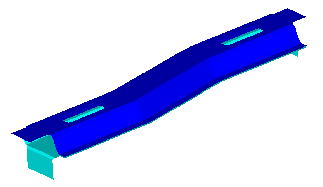
Figure 2.The spot welds are modelled with CBAR elements between the two plates.
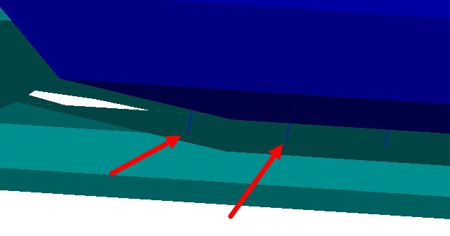
Figure 3.
Tip: Quickly import the model by dragging and
dropping the .h3d file from
a windows browser into the HyperLife
modeling window.
Define the Fatigue Module
-
Click the arrow next to the fatigue module icon and select the
Weld tool from the list of options.

Figure 4.The Weld dialog opens. -
Accept the default parameters.
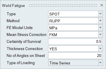
Figure 5.
Assign Materials
-
Click the Material tool.

Figure 6.The Assign Material dialog opens. -
Click
 .
A new material named Mat_WELD("n") is created.
.
A new material named Mat_WELD("n") is created. -
Click Plot & Save.
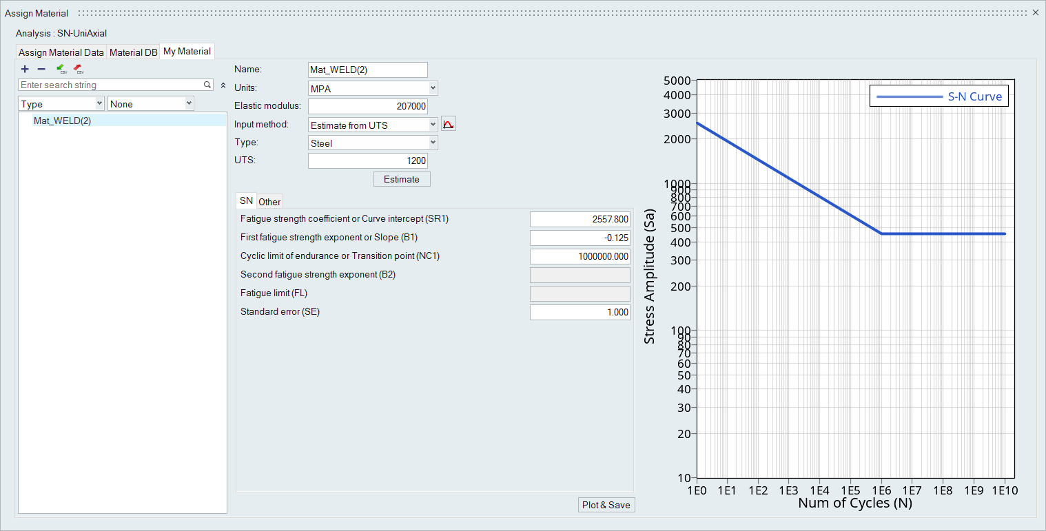
Figure 7. -
For both groups, enter a value of 8.0 for the
Thickness/Diameter of Nugget.
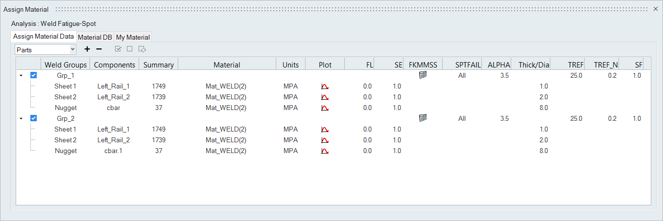
Figure 8.
Assign Load Histories
-
Click the Load Map tool.

Figure 9.The Load Map dialog opens. -
Click to add the load case.
Tip: Click
 to view a plot of the load.
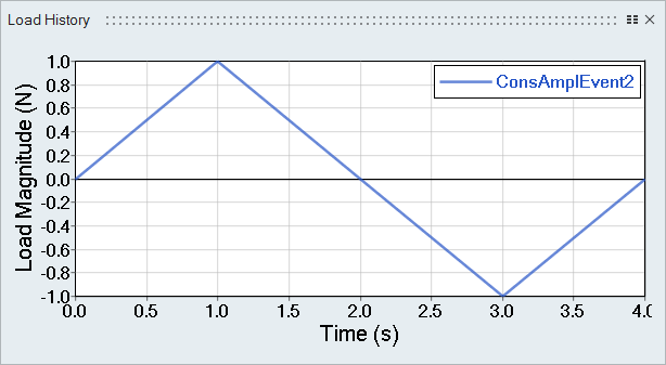
Figure 10. -
Select both Subcase 1 and
ConsAmpEvent1 and click next to Single Event.
An Event_1 header is created.
-
Select Subcase 2 and
ConsAmpEvent1 and click .
An Event_2 header is created.
-
Right click on the Scale and LDM
fields for Subcase 1 and select Apply value to all
events.
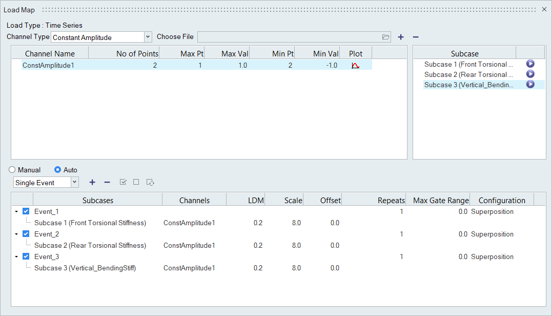
Figure 11.
Evaluate and View Results
-
From the Evaluate tool group, click the
Run Analysis tool.

Figure 12.The Evaluate dialog opens.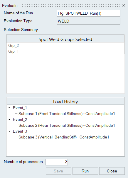
Figure 13. -
Use the Results Explorer to
visualize various types of results.
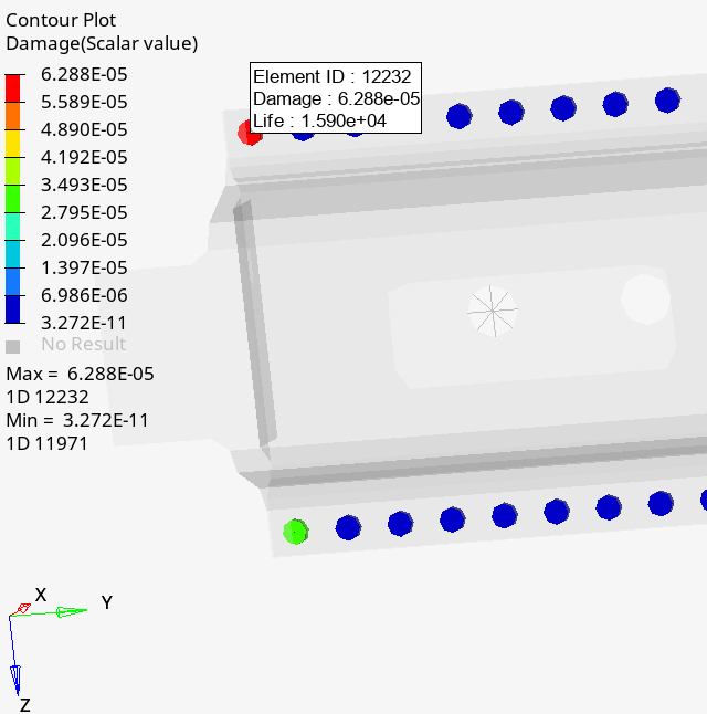
Figure 14.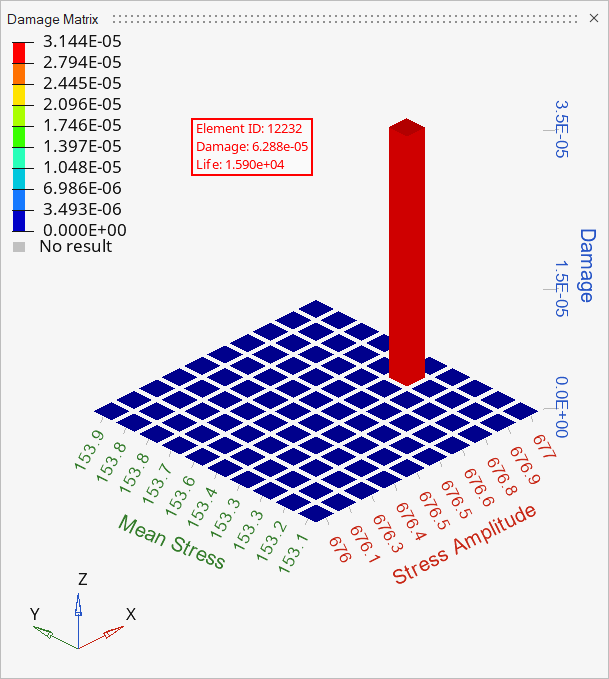
Figure 15.The life of the critical spot weld is around 1.591e4 cycles.