Flux-Portunus co-simulation: preparation of the Portunus model
Introduction
Now that the preparation for the Flux project has been done, the preparation of the Portunus model can be carried out.
Upon the opening of Portunus, the user must prepare the Portunus model by adding and characterizing the Flux coupling component and equally the necessary libraries for the construction of the desired model.
Portunus library
The next figure shows the location of the Flux coupling component available in the Portunus library so called “ Interfaces ” library:
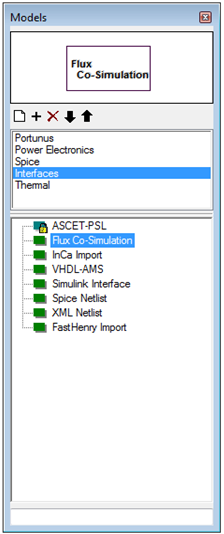
| Element | Function |
|---|---|
| Interfaces Library | Library that contains the Flux – Portunus couplings component. This library is directly accessible with the panel Portunus models. |
| Coupling component |
Permits the coupling between Flux and Portunus. In order to use it, just drag & drop the coupling component into Portunus Sheet. This section is compatible with the new Flux 2D, Flux 3D and Flux Skew on the 32 and 64 Bits system. |
« Flux Co-Simulation » block
The new block «Flux Co-Simulation» available in Portunus has several properties which are classified as follow:
- The coupling file (*.F2P)
- The algorithm « Fast » or « High
precision »
- Fast algorithm option: Maximum input variation (%)
- Both algorithms option: Stops
- Extrapolation « linear » or « Quadratic »
- Flux parameters
- Step Size (s)
- Memory (MB)
- CPU: 32 bit or 64bit
The content of each of these tabs is detailed in the following sections.
"Flux Co-Simulation" component
Here is the content of the “Flux Co-Simulation component”:
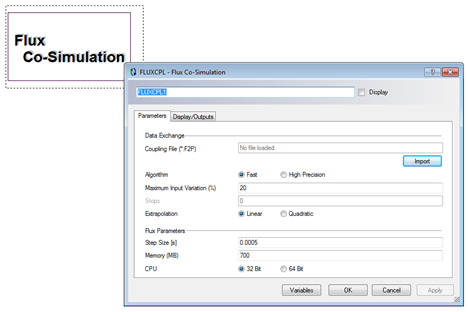
"Parameter" Tab
Here are the contents of the "Parameter" tab:
| Element | Function |
|---|---|
| Coupling File (*.F2P) | Permits the user to point on the coupling file *.F2P (Flux to Portunus) by clicking on “ import ” button. It will ensure the coupling between the Flux project (named ComponentNameF2P.FLU ) and this Portunus project. |
| Algorithm |
Two alternative methods for exchanging data between Flux and Portunus are available and may be selected in the coupling component dialog in Portunus with “Fast” or “high precision”.
Note: More information could be found in the document
“Flux-Portunus Co-Simulation.pdf” in the
installation directory of Portunus
|
|
Maximum Input Variation value (%) |
This option is available when the “Fast” coupling method is chosen: the Maximum Input Variation value allows for forcing a Flux run instead of performing an extrapolation although the time of the next Flux step has not been reached yet. This parameter defines the accepted relative difference (percentage) between the Flux input values of the last and present time step. If the calculated difference exceeds this value, the extrapolation of the output values is regarded as useless and therefore a Flux run is forced. |
| Stops | For both coupling methods the option of defining parameter ranges can be used: The “Stops” field of the wizard allows for the definition of limitations on the Flux inputs. This can be useful in cases like mechanical limits (e.g. air gap length) where an intersection of two bodies must be prevented. In most of the cases the limitation can be done in the Portunus model, but the rejection of numerical deviations may improve the stability of coupled simulations. |
| Extrapolation |
During the simulation, Flux is called according to the step size values set in the coupling model wizard. If Portunus performs smaller steps, extrapolations of the Flux outputs are performed. In order to have as much flexibility as possible, either linear or quadratic extrapolation method can be chosen in the wizard of the coupling model.
|
| Step Sizes | This is the step size used in the scenario of the Flux project. Different step sizes may be used for simulation steps of Portunus and Flux. While a Flux calculation can be done only if Portunus calculates a step, Portunus may calculate its equation without calling Flux. A specific Flux step size can be specified if the system modeled in Portunus requires smaller step sizes than the system modeled in Flux. |
| Memory (MB) | Flux numerical memory can be changed in the same way as in the Flux Supervisor. |
| CPU | One can choose either 32 bits or 64 bits Flux version (if available). |

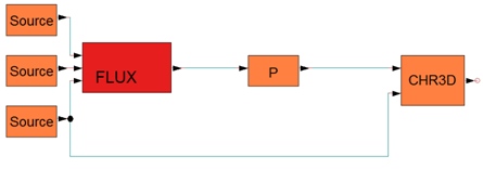
When the field of the path file .F2P is filled, and after clicking on “OK”, the component coupling is turning on red and pins connection appears as follow:
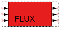
On the left side of the component are « input » parameters; on the right side are « output » parameters.
Input and Output pins connections are defined as “ non conservative ” pins, it means pins could link with a wire only with non conservative block available in Portunus library. Below is an example:
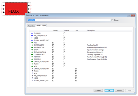
"Display/Outputs" Tab
Here are the contents of the « Display/Outputs » tab:
Inputs and outputs of the coupling model are available as for every other Portunus component. It allows to display curves of each parameters (input/output) of the coupling component in Portunus “off sheet display”.
An additional output called “FLUXRUN” is added to visualize at what time and how often Flux has been run during the simulation.