Flux-Portunus co-simulation: example
Introduction
To permit to the user to implement the co-simulation between Flux and Portunus, a detailed example, with the main stages to be implemented, is given in the following sections.
Example description
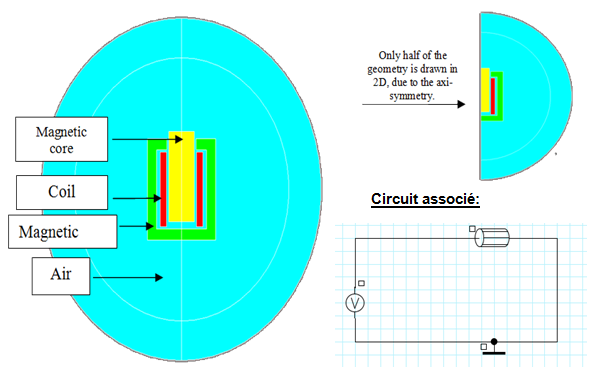
The example represents the behavior of an electromagnetic actuator. The magnetic part of the actuator is designed with the finite element method via Flux 2D software and axisymmetric application. The electric drive and the mechanical part are designed with Portunus software.
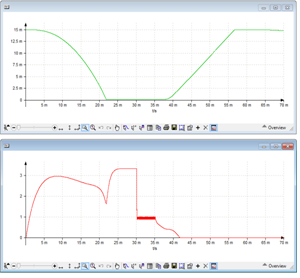
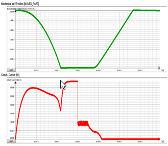
The aim is to observe different operating phase of this actuator with one transient simulation: closing phase, current regulation and opening phase.
Flux project
The geometry, mesh and physics are given below.
Preparation of I/O parameters in Flux
The input and output parameters are described as follows:
| I/O | name | Description | Type | Value / formula |
|---|---|---|---|---|
| Input parameters | LINPOS_MOVED_PART | Linear position (m) of mechanical set “MOVED_PART” which represents the position of the magnetic core of the plunger. This parameter is automatically created in the case of mechanical set with at type of kinematics “MultiphysicsPosition” |
I/O parameter, multiphysics |
Reference value = 0 |
| R_BOB | Parameter associated to the resistance of the stranded coil in the electrical circuit: for example it is possible to do a parametric analysis under Portunus on this electrical parameter (this value is fixed during a transient analysis). |
I/O parameter, multiphysics |
Reference value = 10 | |
| V_IN | Supply voltage of the coil associated to the voltage source Source V1 |
I/O parameter, multiphysics |
Reference value = 0 | |
| Output parameters | AIR_GAP_POSITION | Represent the position of the magnetic core with an offset | I/O parameter defined by a formula | LinPos(MOVED_PART)+ 15/1000 |
| I_BOB | Current in the stranded coil B2 | I/O parameter defined by a formula | I(B2) | |
| ELFORC_MOVED_PART | Magnetic force measured on the Mechanical set “MOVED_PART” | I/O parameter defined by a formula | ForceElecMag(MOVED_PART) |
Generation of the coupling file from Flux
Here are the steps to generate the coupling file F2P from Flux:
| Step | Actions |
|---|---|
| 1 |
Open the dialog box:
|
| 2 | Define the name of component ( for example COMPONENT_COSIM) |
| 3 |
Choose the input parameters:
|
| 4 |
Choose the output parameters:
|
| 5 | Validate by clicking on OK |
| → |
A COMPONENT_COSIM.F2P file has been created. The Flux project has been duplicated and registered under the name: COMPONENT_COSIMF2P.FLU |
Preparation of the Portunus model
To prepare the Portunus model:
| Step | Actions |
|---|---|
| 1 | Open Portunus by clicking on |
| → | The main interface of Portunus is opened. |
| 2 |
Register the model:
|
| 3 |
Go in the Models library « Interfaces »:
|
| 4 |
Characterize the “Flux Co-Simulation” component:
|
| → | The Inputs/Outputs ports appear and the coupling component become red. |
| 5 |
By selecting check box, choose “outputs” that you want to analyze in the Portunus off-sheet display. |
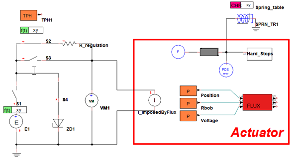
| 6 | Place, characterize and connect the other necessary components (which is the environment of the electromagnetic actuator) according to the model in the figure below. |
| 7 | Save the model by clicking on Save in the menu File |
| → | The preparation of the Portunus model is complete. |
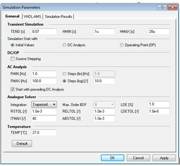
Simulation configuration
Configure the simulation parameters with a time interval from 0 to 70ms and the time step set between 1µs and 20µs and launches the solving process.
During the solving process the information on the solved steps are displayed in the off-sheet display of Portunus.
Analysis of results
The results can be analyzed in Portunus, as well as from Flux in the project COMPONENT_COSIMF2P.FLU
| Graph results in Portunus | Graph results in Flux |
|---|---|
|
|