Calculate propagation between two moving cars in a suburban scenario.
Model Type
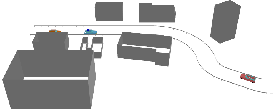
Two moving cars in a suburban scenario are modeled with the transmitter mounted on
the roof of the blue car. All cars are moving in this scenario. As the transmitter
is mounted on one of the cars, it is also time-variant.
Figure 1. Model of suburban structures and topography.
Sites and Antennas
The antenna is mounted on the roof of a moving car at a height of 1.8 m. The database
for this time-dependent moving car is defined in WallMan. The antenna is an omnidirectional antenna at 3.4 GHz.
Computational Method
This project uses the 3D ray tracing (SRT) model to determine the
propagation path and received signal for each receiver signal in the scenario.
Tip: Click Project > Edit Project Parameter and click the Computation tab to change
the model.
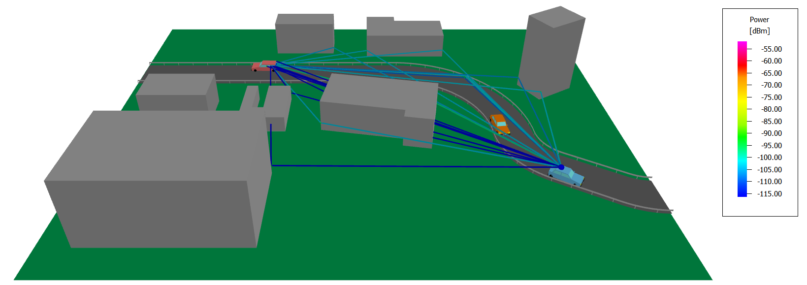
The method considers reflections and diffraction. Some propagation paths are shown
between the transmitter and a receiver location near the orange car. The ray file
(.str) was removed from the
example and needs to be recomputed).
Figure 2. Propagation ray paths for the power results for time stamp 6 s.
Results
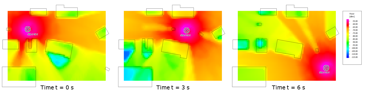
The results are computed for six timestamps in this model, from 0 s to 6 s in steps
of 1 s. Results for different time steps can be viewed in the Edit toolbar from the
Floor Levels above Grounddrop-down list.
The received signal power is displayed for three different timestamps, see Figure 3.
Figure 3. Received signal power for three different timestamps.