Fatigue Process Manager (FPM) using E-N (Strain - Life) Method
The E-N (Strain - Life) method should be chosen to predict the fatigue life when plastic strain occurs under the given cyclic loading. S-N (Stress - Life) method is not suitable for low-cycle fatigue where plastic strain plays a central role for fatigue behavior.
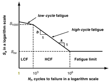
Figure 1. Low Cycle and High Cycle regions on the S-N curve
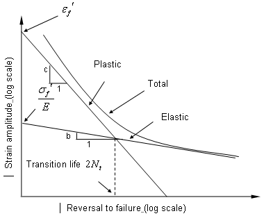
Figure 2. Strain-Life Curve
In OptiStruct, various strain combination types are available with the default being "Absolute maximum principle strain". In general "Absolute maximum principle stain" is recommended for brittle materials, while "Signed von Mises strain" is recommended for ductile material. The sign on the signed parameters is taken from the sign of the Maximum Absolute Principal value.
In this tutorial, you will be able to evaluate fatigue life with the E-N method.
The following files found in the optistruct.zip file are needed to perform this tutorial. Refer to Access the Model Files.
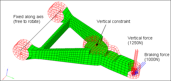
Figure 3. Model of Control Arm for Fatigue Analysis
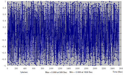
Figure 4. Load Time History for Vertical Force
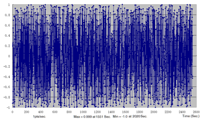
Figure 5. Load Time History for Braking Force
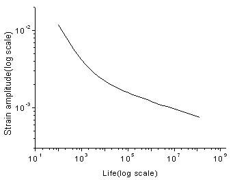
Figure 6. E-N Curve of Aluminum
Launch HyperMesh and Process Manager
-
Click Create.
This creates a new file to save the instance of the currently loaded fatigue process template.

Figure 7.
Import the Model
-
Click the Open model file icon
 .
A Select File browser window opens.
.
A Select File browser window opens. -
Click Apply.
This guides you to the next task Fatigue Subcase of the Fatigue Analysis tree.

Figure 8. Import a Finite Element Model file
Set Up the Model
Create a Fatigue Subcase
-
Click Apply.
This saves the current definitions and guides you to the next task Analysis Parameters of the Fatigue Analysis tree.

Figure 9. Create and Select Active Fatigue Subcase to Process
Apply Fatigue Analysis Parameters
-
Click Apply.
This saves the current definitions and guides you to the next task Elements and Materials of the Fatigue Analysis tree. For details, consult the Altair Simulation 2021.2 help.

Figure 10. Fatigue Analysis Parameters Definition
Add Fatigue Elements and Materials
-
For Input method of Define EN Curve, select Estimate From
UTS.

Figure 11. Material Data Definition -
Click the Show EN curve definition icon
 .
An EN method description window introducing how to generate the EN material parameter opens.
.
An EN method description window introducing how to generate the EN material parameter opens. -
Click Save to save the definition of the EN data for the
selected entities.

Figure 12. -
Click Apply.
This saves the current definitions and guides you to the next task Load-Time History of the Fatigue Analysis tree.
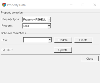
Figure 13. Material Data Definition
Figure 14. Elements and Material Definition
Add Load-Time History
-
Click the Open load-time file icon .
An Open file browser window opens.
-
Create another load-time history named lth2 by importing
the file load2.csv.
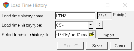
Figure 15. Import Load-Time History -
Click Apply.
This saves the current definitions and guides you to the next task Loading Sequences of the Fatigue Analysis tree.
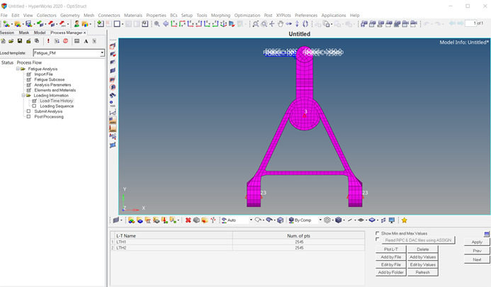
Figure 16. Load-time History DefinitionNote: For a file of DAC format, it can very easily be imported in HyperGraph and converted to CSV format for use by FPM.
Load Sequences
-
Click + to create a single event with two subcases and
two channels.

Figure 17. Load Mapping to associate load-time history with static subcase -
Click Save to close the window and create the fatique
event using selected subcases and channels.
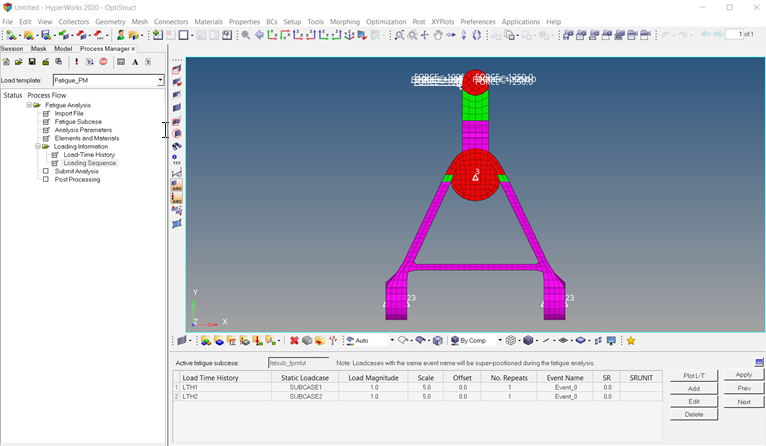
Figure 18. Loading Sequences Definition
Submit the Job
-
Click the Save .fem file icon .
A Save As browser window opens.
-
Click Submit.
This launches OptiStruct 2021.2 to run the fatigue analysis. If the job is successful, the new results files should be in the directory from which was selected.The default files written to the directory are:
ctrlarm_fpmtut.0.3.fat An ASCII format file which contains fatigue results of each fatigue subcase in iteration step. ctrlarm_fpmtut.h3d Hyper 3D binary results file, with both static analysis results and fatigue analysis results. ctrlarm_fpmtut.out OptiStruct output file containing specific information on the file set up, the set up of your fatigue problem, compute time information, etc. Review this file for warnings and errors. ctrlarm_fpmtut.stat Summary of analysis process, providing CPU information for each step during analysis process. Note: The filename.#.fat is created for each fatigue subcase at the first and last iterations only if a fatigue optimization is performed.
Figure 19. Submit Fatigue Analysis
Post-process the Analysis
-
Click Exit to unload Fatigue Process Manager.

Figure 20. Post-Processing
Figure 21. Damage Contour in HyperView