In this tutorial you will setup an optimization problem using MotionSolve's Optimization Wizard for a 4-bar model.
You will learn about the following:
Defining point coordinates as design variables
Defining a response type 'Root Mean Square Deviation' for matching curves
Using the responses as objectives
Running the optimization and post-processing the results
[Optional] Infeasible Designs in MotionSolve
optimization
Introduction
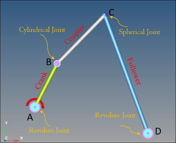
In this tutorial, the locations of the joints of a 4-bar mechanism are
optimized to obtain a desired motion of the coupler. MotionSolve's DSA (Design Sensitivity Analysis)
capability is used to calculate sensitivities. Figure 1. 4 bar model with joint types
The entire model is parameterized in terms of these four design
points: A, B, C and D. Since the model operates in 2D space (X-Y plane),
this leads to 8 Design Variables. The initial design is listed as in Table 1:
Table 1.
Point
X
Y
A
-45
45
B
65
260
C
300
500
D
515
-85
Review the Model
In this step, you will review the 4-bar model in MotionSolve.
Before you begin, copy the file
mv_3022_initial_4bar_opt.mdl located in the
mbd_modeling\motionsolve\optimization\MV-3022 into your
<working directory>.
Open the file mv_3022_initial_4bar_opt.mdl in MotionSolve.
Review the entities in the model.
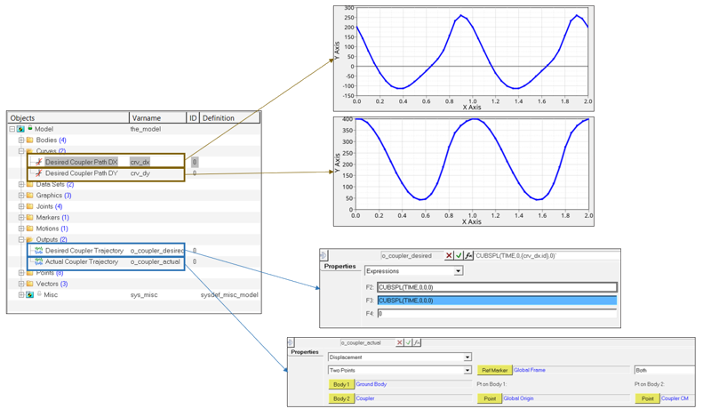
Verify the presence of curves Desired Coupler Path
DX and Desired Coupler Path DY,
which define the desired motion in the X and Y directions.
Verify the presence of output Desired Coupler
Trajectory, which uses the curves to measure the desired
motion.
Verify the presence of output Actual Coupler
Trajectory, which measures the displacement of the
coupler body at the CM.
Figure 2.
Add Design Variables
In the Project Browser, right-click on
Model and select Optimization
Wizard from the context menu.
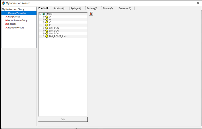
In the Design Variables page, click on the
Points tab.
The points are listed in Figure 3: Figure 3. Optimization Wizard – Points Tab
For points A, B, C, and D, make the x and y coordinates design variables. Click
the (Filter datamembers) icon.
In the Filter dialog, click to turn off the
Z check box.
Figure 4.
Click OK.
In the Model Tree, select Point
A, Point B, Point
C, and Point D. Then click
Add.
Modify the upper and lower bounds of the design variables according to Table 2:
Table 2.
DV
Lower Bound
Upper Bound
Point A(DV) - X
-50
50
Point A(DV) - Y
-50
50
Point B(DV) - X
20
80
Point B(DV) - Y
180
280
Point C(DV) - X
240
380
Point C(DV) - Y
400
620
Point D(DV) - X
180
520
Point D(DV) - Y
-100
20
You have finished the process of setting design variables.
Add Response Variables
Now you will add response variables to the optimization.
The objective of this optimization is to make the coupler move along a path. To
achieve this, you will add two responses:
Trajectory of Coupler CM – DX
Trajectory of Coupler CM – DY
The above curves of the coupler motion must be matched with their respective target
curves using a response variable of type Root Mean Square Deviation (RMS2). The details
of this response can be obtained from the Multibody Optimization User’s
Guide and the MotionView User’s Guide.
Click on the Responses page.
Click on the button.
Change the Label to 'rms2_dx'.
Click OK to create a response
variable.
Once the response variable is created, under Response Type, choose
Root Mean Square Deviation.
Double-click the Curve collector and choose
Desired Coupler Path DX for the Desired Curve user
input. This is the target curve for Couple-DX.
For Response Expression, type the expression
`DX({b_bc.cm.id})` (DX of CM coupler body).
Follow the steps again to create one more Root Mean Square
Deviation response. Use Table 3 to fill in the
details.
Table 3.
RV
Desired Curve
Response Expression
rms2_dx
Desired Coupler Path DX
`DX({b_bc.cm.id})`
rms2_dy
Desired Coupler Path DY
`DY({b_bc.cm.id})`
The completed Responses page should appear as shown
in Figure 5: Figure 5. Completed Responses page
Add Objectives and Constraints
In this step you will add two objectives to the problem.
The objectives of the problem are as follows: the coupler DX and DY motions should
match with target curves at the end of optimization. You can use the responses that were
created in the previous section as objectives.
Navigate to the Goals page.
Under Objectives, click .
This will add an objective with the response rv_rms2_dx.
For Weight choose 1.0 retain the Type as
min (you want to minimize the response).
Repeat these steps to add another objective. Choose
rv_rms2_dy for the second objective.
For Weight choose 1.0 retain the Type as
min.
There are no constraints in this problem, so you have now finished model
setup. The model is ready to solve. Figure 6. Defining objectives
Run the Optimization
Now you will run the optimization.
Navigate to the Solutions page.
Activate the Plot Optimization Summary check box.
Click on Save & Optimize to start the
optimization.
Once the optimization process is complete, the text window displays the
optimized design variables values, final value of the responses and optimized
cost function. Figure 7. Optimization text window after the optimization is completed
The expected values of design variables are provided in Table 4:
Table 4.
DV
Expected
From Optimizer
p_0.x
0
-0.0660
p_0.y
0
-0.2796
p_1.x
40
39.97
p_1.y
200
199.71
p_2.x
360
360.07
p_2.y
600
600.26
p_3.x
400
400.44
p_3.y
0
-0.0406
Post-Process
In this step you will post-process the results of the optimization run.
Once the solution is finished, navigate to the Review
Results page.
The Summary tab lists the history of design variables,
responses and objective functions in a tabular format. In this tutorial, the
optimized design variables are from iteration 27. Figure 8. Summary tab listing design variables, responses and cost function
iteration-wise
Click the Plot tab. Plot Overall
Objective versus Iteration
variable.
The Plot tab helps to visualize variation of design
variables, response variables and cost function using graphs. You can choose to
plot any number of variables along the y-axis with respect to a variable along
the x-axis. Figure 9. Plot of overall objective (log scale) vs. iteration number
Note: You can also see how a particular design variable varied across an
iteration. For example, select p_b.x (Point B-X) in
the Y list and click Apply. Figure 10.
Animate the configuration generated during any iteration.
In the Animation tab, from the Iteration
drop-down menu choose the iteration number you want to animate (for this
tutorial, choose Iteration 27.
Click Load Result to load the animation
corresponding to the iteration you chose.
Figure 11. Animation tab in the Post Processing page
From this tab, you also have the option to export an archive of the model
from any configuration.
Load the results from Iteration 27.
Use the Archive Model location browser to choose a file
path.
Click Export.
Observe how the path of the coupler for the optimized result compares with the
desired target path.
Close the Optimization Wizard.
Add a page to your MotionView
session.
Change the client in the new page to HyperGraph.
Open the .abf file in the last iteration folder of
the optimization run.
Note: The optimization run directory is automatically created during the
solution and follows the naming convention
py_name_timestamp where
py_name is the name of the Python file given in the Solution page and
timestamp is the time when the solution was initiated. Figure 12.
For the X and Y axis, select the following Type,
Request, and
Component:
Table 5.
Axis
Type
Request
Component
X
Expressions
REQ/70000000 Desired Coupler Trajectory
F2
Y
Expressions
REQ/70000000 Desired Coupler Trajectory
F3
Figure 13.
Click Apply.
Plot the actual trajectory of the coupler CM using the following X and
Y axis specifications:
Table 6.
Axis
Type
Request
Component
X
Marker Displacement
REQ/70000003 Actual Coupler Trajectory - (on
Coupler) (on 'Coupler')
X
Y
Marker Displacement
REQ/70000003 Actual Coupler Trajectory - (on
Coupler) (on 'Coupler')
Y
The resulting plots will overlay each other. Figure 14.
In this step, you will use a powerful feature in MotionSolve to obtain the optimal design by recovering from a failed
iteration.
It is not uncommon for a mechanical system to be limited by some sort of physical
constraints. In this four bar example, the Grashof constraints have to be satisfied
in order to make the input link a crank. When optimizer chooses a new design, those
constraints are likely to be violated regardless of whether they are added as
optimization constraints or not. The optimizer in MotionSolve has a recovery mode to help recover from such
infeasible design and let optimization proceed. To demonstrate how the optimizer
recovers in this tutorial, you will change the initial design and see how it
works.
Return to the Design Variables page and change the
nominal value, upper and lower bounds as shown in Figure 15:
Figure 15. Value of Design Variables
The four bar mechanism should look like the example in Figure 16: Figure 16. Four bar mechanism after changing the value of Dvs
Retain the Responses, Objectives and Constraints you defined earlier in the
tutorial.
Run an optimization with a different Output file in the Solutions page as
4bar_opt_for_recover.py.
The number of iterations will change due to a different initial design.
Important: Pay attention to the last column ‘Reduced Step’ in the
solver output: Figure 17. Solver output when recovery mode is invoked
In this example, the optimizer has found infeasible design in
iteration 2-7; it is then told to reduce the step size until a feasible design
is found.
Check the output files. In most cases, the output files could tell you why
solver fails at a specific point and how you can avoid it if possible.
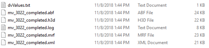
Figure 18. Subfolders that contain the infeasible designs
When the optimizer recovers from an infeasible design, an additional
folder ‘Infeasible Points’ is created; each subfolder
contains the following information:
dvValues.txt: Value of design variables
4bar_opt_for_recover.abf: MotionSolve output
file
4bar_opt_for_recover.h3d: Animation file (provided only when
available)
4bar_opt_for_recover.log: MotionSolve log
file
4bar_opt_for_recover.mrf: MotionSolve output
file
4bar_opt_for_recover.xml: MotionSolve xml
input file
Figure 19. Output for each infeasible design
You have found that the h3d file and log file are useful in most cases.
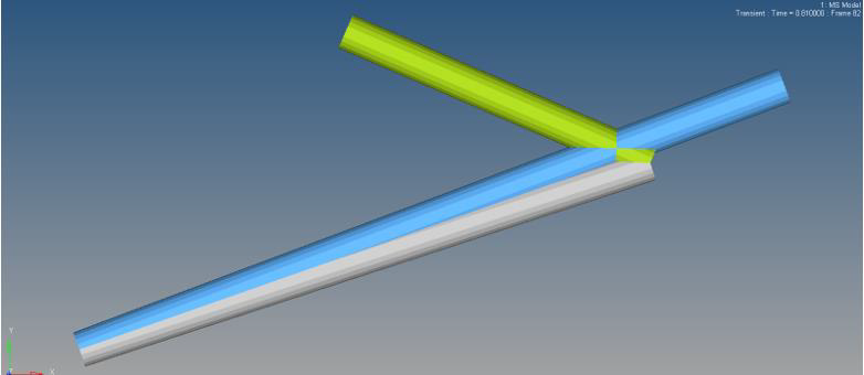
You will load this h3d file in HyperView and see
what is going wrong.
Load 4bar_opt_for_recover.h3d in folder
Infeasible Point 1 -- iter-2.
You can see that the system enters a lock-up position before the solver
crashes: Figure 20.
Check the result.
The result you see in the example is very close to what you get in STEP 5 and
the cost function is reduced significantly. This shows you can get the
optimal design even with infeasible design encountered in the intermediate
step. However, the optimality is not guaranteed in some cases. When that
happens, you can improve the result by adding proper constraints based on
your investigation in previous steps. For four bar mechanism, you can add
Grashof constraints. An example of how to do this in MotionSolve is included.
 (Filter datamembers) icon.
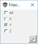 Figure 4.
  button.
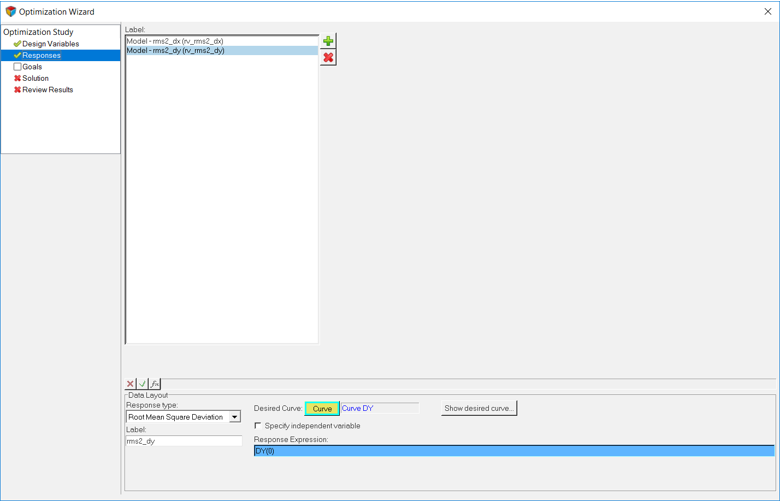
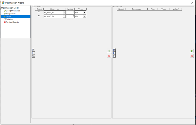
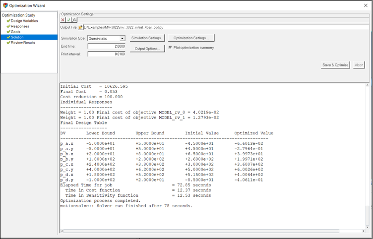
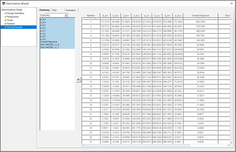
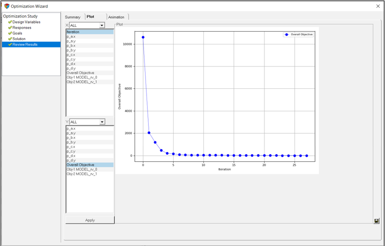
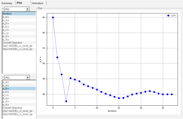
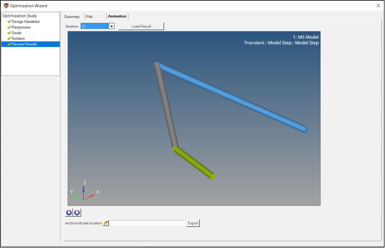
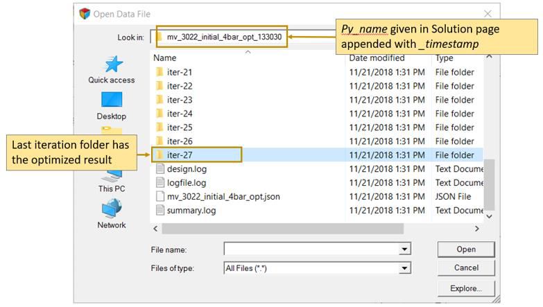
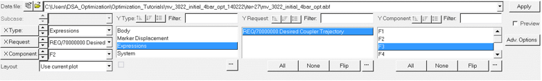
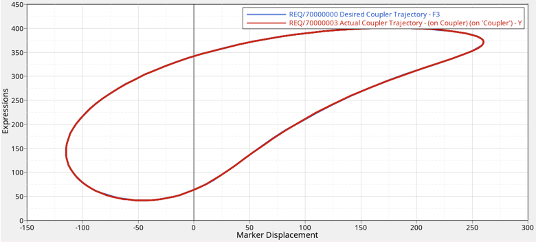
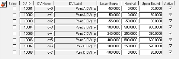
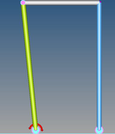
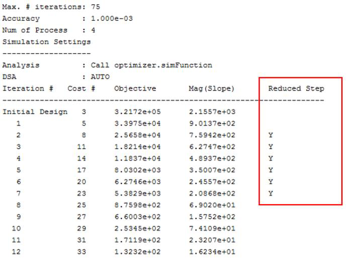
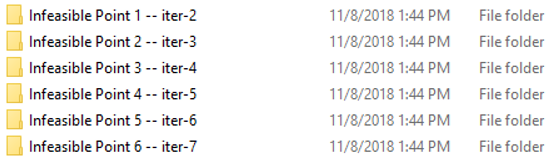 Figure 18. Subfolders that contain the infeasible designs