Glossary

Term
Definition
Conjugate Gradient
An iterative algorithm for the numerical solution of symmetric and positive-definite systems of linear equations. A key feature of this algorithm is that the direction at step K is conjugate (A-orthogonal) to the directions at all the previous steps.
Constrained Optimization
Constrained optimization is the process of optimizing (usually minimizing) an objective function with respect to some design variables in the presence of constraints on those designs variables. These constraints can be bounds on the design space, equality constraints and inequality constraints. The sought after solution is required to satisfy all the constraints.
Constraints
Constraints are algebraic relationships amongst the design variables that a solution for the optimization must satisfy. The algebraic relationships come in 3 flavors:
  • Simple bound constraints
  • Equality or bilateral constraints
  • Inequality or unilateral constraints
Cost Function
Often called the objective function, this is the quantity that is to be minimized in an optimization process.
Design Bound Constraints
These specify lower bounds (bL) and upper bounds (bLon the design parameters that the solution is required to satisfy. Thus at any feasible design point b*, bL≤ b* ≤ bU
Design Variables
These are the quantities that are to be determined in the optimization problem. In the CAE context, design variables are used to define parametric models. By changing the values for design variables in a model, you can change the model. An optimizer will change the values of the design variables for a model in its quest to find an optimum solution.
Equality Constraints
A set of nonlinear or linear algebraic equations that the solution must satisfy. The equality relationships are usually expressed in the form
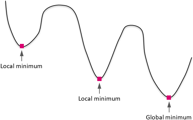
 ψ k ( b ) + t 0 t f L k ( x , b , t ) d t = 0 k = p + 1 m MathType@MTEF@5@5@+= feaagKart1ev2aqatCvAUfeBSjuyZL2yd9gzLbvyNv2CaerbdfgBPj MCPbqefqvATv2CG4uz3bIuV1wyUbqeduuDJXwAKbYu51MyVXgaruWq VvNCPvMCG4uz3bqeeuuDJXwAKbsr4rNCHbGeaGqiFu0Je9sqqrpepC 0xbbL8F4rqqrFfpeea0xe9Lq=Jc9vqaqpepm0xbba9pwe9Q8fs0=yq aqpepae9pg0FirpepeKkFr0xfr=xfr=xb9adbaGaaiGadmWaamaaci GaaqqaceqbcaGcbaGaeqiYdK3aaSbaaSqaaiaadUgaaeqaaOGaaiik aiaadkgacaGGPaGaey4kaSYaa8qCaeaacaWGmbWaaSbaaSqaaiaadU gaaeqaaOWaaeWaaeaacaWG4bGaaiilaiaadkgacaGGSaGaamiDaaGa ayjkaiaawMcaaiaadsgacaWG0baaleaacaWG0bGaaGimaaqaaiaads hacaWGMbaaniabgUIiYdGccqGH9aqpcaaIWaGaae4oaiaabccacaWG RbGaeyypa0JaamiCaiabgUcaRiaaigdacqGHMacVcaWGTbaaaa@5CD6@
Global Optimization
An optimization process wherein the global minimum of a function is sought. Let f() be the function being minimized, and b the design variables. A solution b* is said to be a global minimum if f (b*) ≤ f (b) for all b ≠ b*.


Gradient
If f(x1, ..., xn) is a differentiable, real-valued function of several variables, its gradient is the vector whose components are the n partial derivatives of f.
grad ( f ) = [ f x 1 f x 2 f x n ] T MathType@MTEF@5@5@+= feaagKart1ev2aqatCvAUfeBSjuyZL2yd9gzLbvyNv2CaerbdfgBPj MCPbqefqvATv2CG4uz3bIuV1wyUbqeduuDJXwAKbYu51MyVXgaruWq VvNCPvMCG4uz3bqeeuuDJXwAKbsr4rNCHbGeaGqiFu0Je9sqqrpepC 0xbbL8F4rqqrFfpeea0xe9Lq=Jc9vqaqpepm0xbba9pwe9Q8fs0=yq aqpepae9pg0FirpepeKkFr0xfr=xfr=xb9adbaGaaiGadmWaamaaci GaaqqaceqbcaGcbaGaae4zaiaabkhacaqGHbGaaeizamaabmaabaGa amOzaaGaayjkaiaawMcaaiabg2da9maadmaabaqbaeqabeabaaaaba WaaSaaaeaacqGHciITcaWGMbaabaGaeyOaIyRaamiEamaaBaaaleaa caaIXaaabeaaaaaakeaadaWcaaqaaiabgkGi2kaadAgaaeaacqGHci ITcaWG4bWaaSbaaSqaaiaaikdaaeqaaaaaaOqaaiablAcilbqaamaa laaabaGaeyOaIyRaamOzaaqaaiabgkGi2kaadIhadaWgaaWcbaGaam OBaaqabaaaaaaaaOGaay5waiaaw2faamaaCaaaleqabaGaamivaaaa aaa@5995@
Hessian Matrix
The Hessian matrix or Hessian is a square matrix of second-order partial derivatives of a scalar-valued function, or scalar field. It describes the local curvature of a function of many variables. The Hessian matrix was developed in the 19th century by the German mathematician Ludwig Otto Hesse and later named after him. The Hessian matrix  H  of  f ( x 1 , x n )  is a square  n × n  matrix, computed as: H = [ 2 f x 1 2 2 f x 1 x 2 2 f x 1 x n 2 f x 2 x 1 2 f x 2 2 2 f x 2 x n 2 f x n x 1 2 f x n x 2 2 f x n 2 ] MathType@MTEF@5@5@+= feaagKart1ev2aaatCvAUfeBSjuyZL2yd9gzLbvyNv2CaerbdfgBPj MCPbqefqvATv2CG4uz3bIuV1wyUbqeduuDJXwAKbYu51MyVXgaruWq VvNCPvMCG4uz3bqeeuuDJXwAKbsr4rNCHbGeaGqiFu0Je9sqqrpepC 0xbbL8F4rqqrFfpeea0xe9Lq=Jc9vqaqpepm0xbba9pwe9Q8fs0=yq aqpepae9pg0FirpepeKkFr0xfr=xfr=xb9adbaGaaiGadmWaamaaci GaaqqaceqbcaGceaqabeaaqqaaaaaaaaGySf2yRbWdbiaabsfacaqG ObGaaeyzaiaabccacaqGibGaaeyzaiaabohacaqGZbGaaeyAaiaabg gacaqGUbGaaeiiaiaab2gacaqGHbGaaeiDaiaabkhacaqGPbGaaeiE aiaabccacaWGibGaaeiiaiaab+gacaqGMbGaaeiiaiaadAgadaqada qaaiaadIhadaWgaaWcbaGaaGymaaqabaGccaGGSaGaeSOjGSKaamiE amaaBaaaleaacaWGUbaabeaaaOGaayjkaiaawMcaaiaabccacaqGPb Gaae4CaiaabccacaqGHbGaaeiiaiaabohacaqGXbGaaeyDaiaabgga caqGYbGaaeyzaiaabccacaWGUbGaey41aqRaamOBaiaabccacaqGTb GaaeyyaiaabshacaqGYbGaaeyAaiaabIhacaqGSaGaaeiiaiaaboga caqGVbGaaeyBaiaabchacaqG1bGaaeiDaiaabwgacaqGKbGaaeiiai aabggacaqGZbGaaeOoaaqaaiaadIeacqGH9aqpdaWadaqaauaadeqa eqaaaaaabaWdamaalaaabaGaeyOaIy7aaWbaaSqabeaacaaIYaaaaO GaamOzaaqaaiabgkGi2kaadIhadaqhaaWcbaGaaGymaaqaaiaaikda aaaaaaGcpeqaa8aadaWcaaqaaiabgkGi2oaaCaaaleqabaGaaGOmaa aakiaadAgaaeaacqGHciITcaWG4bWaaSbaaSqaaiaaigdaaeqaaOGa eyOaIyRaamiEamaaBaaaleaacaaIYaaabeaaaaaak8qabaGaeSOjGS eabaWdamaalaaabaGaeyOaIy7aaWbaaSqabeaacaaIYaaaaOGaamOz aaqaaiabgkGi2kaadIhadaWgaaWcbaGaaGymaaqabaGccqGHciITca WG4bWaaSbaaSqaaiaad6gaaeqaaaaaaOWdbeaapaWaaSaaaeaacqGH ciITdaahaaWcbeqaaiaaikdaaaGccaWGMbaabaGaeyOaIyRaamiEam aaBaaaleaacaaIYaaabeaakiabgkGi2kaadIhadaWgaaWcbaGaaGym aaqabaaaaaGcpeqaa8aadaWcaaqaaiabgkGi2oaaCaaaleqabaGaaG OmaaaakiaadAgaaeaacqGHciITcaWG4bWaa0baaSqaaiaaikdaaeaa caaIYaaaaaaaaOWdbeaacqWIVlctaeaapaWaaSaaaeaacqGHciITda ahaaWcbeqaaiaaikdaaaGccaWGMbaabaGaeyOaIyRaamiEamaaBaaa leaacaaIYaaabeaakiabgkGi2kaadIhadaWgaaWcbaGaamOBaaqaba aaaaGcpeqaaiabl6Uinbqaaiabl6UinbqaaiablgVipbqaaiabl6Ui nbqaa8aadaWcaaqaaiabgkGi2oaaCaaaleqabaGaaGOmaaaakiaadA gaaeaacqGHciITcaWG4bWaaSbaaSqaaiaad6gaaeqaaOGaeyOaIyRa amiEamaaBaaaleaacaaIXaaabeaaaaaak8qabaWdamaalaaabaGaey OaIy7aaWbaaSqabeaacaaIYaaaaOGaamOzaaqaaiabgkGi2kaadIha daWgaaWcbaGaamOBaaqabaGccqGHciITcaWG4bWaaSbaaSqaaiaaik daaeqaaaaaaOWdbeaacqWIMaYsaeaapaWaaSaaaeaacqGHciITdaah aaWcbeqaaiaaikdaaaGccaWGMbaabaGaeyOaIyRaamiEamaaDaaale aacaWGUbaabaGaaGOmaaaaaaaaaaGcpeGaay5waiaaw2faaaaaaa@E159@
Jacobian Matrix
The Jacobian matrix is the matrix of all first-order partial derivatives of a function f. It is named after the mathematician Carl Gustav Jacob Jacobi (1804–1851).
Let  f ( x 1 , x n ) =   [ f 1 ( x 1 , x n ) f 2 ( x 1 , x n ) f m ( x 1 , x n ) ] T Jacobian  J = [ f 1 x 1 f 1 x 2 f 1 x n f 2 x 1 f 2 x 2 f 2 x n f m x 1 f m x 2 f m x n ] MathType@MTEF@5@5@+= feaagKart1ev2aaatCvAUfeBSjuyZL2yd9gzLbvyNv2CaerbdfgBPj MCPbqefqvATv2CG4uz3bIuV1wyUbqeduuDJXwAKbYu51MyVXgaruWq VvNCPvMCG4uz3bqeeuuDJXwAKbsr4rNCHbGeaGqiFu0Je9sqqrpepC 0xbbL8F4rqqrFfpeea0xe9Lq=Jc9vqaqpepm0xbba9pwe9Q8fs0=yq aqpepae9pg0FirpepeKkFr0xfr=xfr=xb9adbaGaaiGadmWaamaaci GaaqqaceqbcaGceaqabeaaqqaaaaaaaaGySf2yRbWdbiaabYeacaqG LbGaaeiDaiaabccacaWGMbWaaeWaaeaacaWG4bWaaSbaaSqaaiaaig daaeqaaOGaaiilaiablAciljaadIhadaWgaaWcbaGaamOBaaqabaaa kiaawIcacaGLPaaacqGH9aqpcaqGGaWaamWaaeaafaqabeqaeaaaae aacaWGMbWaaSbaaSqaaiaaigdaaeqaaOWaaeWaaeaacaWG4bWaaSba aSqaaiaaigdaaeqaaOGaaiilaiablAciljaadIhadaWgaaWcbaGaam OBaaqabaaakiaawIcacaGLPaaaaeaacaWGMbWaaSbaaSqaaiaaikda aeqaaOWaaeWaaeaacaWG4bWaaSbaaSqaaiaaigdaaeqaaOGaaiilai ablAciljaadIhadaWgaaWcbaGaamOBaaqabaaakiaawIcacaGLPaaa aeaacqWIMaYsaeaacaWGMbWaaSbaaSqaaiaad2gaaeqaaOWaaeWaae aacaWG4bWaaSbaaSqaaiaaigdaaeqaaOGaaiilaiablAciljaadIha daWgaaWcbaGaamOBaaqabaaakiaawIcacaGLPaaaaaaacaGLBbGaay zxaaWaaWbaaSqabeaacaWGubaaaaGcbaGaaeOsaiaabggacaqGJbGa ae4BaiaabkgacaqGPbGaaeyyaiaab6gacaqGGaGaamOsaiabg2da9m aadmaabaqbamqabqabaaaaaeaapaWaaSaaaeaacqGHciITcaWGMbWa aSbaaSqaaiaaigdaaeqaaaGcbaGaeyOaIyRaamiEamaaBaaaleaaca aIXaaabeaaaaaak8qabaWdamaalaaabaGaeyOaIyRaamOzamaaBaaa leaacaaIXaaabeaaaOqaaiabgkGi2kaadIhadaWgaaWcbaGaaGOmaa qabaaaaaGcpeqaaiablAcilbqaa8aadaWcaaqaaiabgkGi2kaadAga daWgaaWcbaGaaGymaaqabaaakeaacqGHciITcaWG4bWaaSbaaSqaai aad6gaaeqaaaaaaOWdbeaapaWaaSaaaeaacqGHciITcaWGMbWaaSba aSqaaiaaikdaaeqaaaGcbaGaeyOaIyRaamiEamaaBaaaleaacaaIXa aabeaaaaaak8qabaWdamaalaaabaGaeyOaIyRaamOzamaaBaaaleaa caaIYaaabeaaaOqaaiabgkGi2kaadIhadaWgaaWcbaGaaGOmaaqaba aaaaGcpeqaaiabl+Uimbqaa8aadaWcaaqaaiabgkGi2kaadAgadaWg aaWcbaGaaGOmaaqabaaakeaacqGHciITcaWG4bWaaSbaaSqaaiaad6 gaaeqaaaaaaOWdbeaacqWIUlstaeaacqWIUlstaeaacqWIXlYtaeaa cqWIUlstaeaapaWaaSaaaeaacqGHciITcaWGMbWaaSbaaSqaaiaad2 gaaeqaaaGcbaGaeyOaIyRaamiEamaaBaaaleaacaaIXaaabeaaaaaa k8qabaWdamaalaaabaGaeyOaIyRaamOzamaaBaaaleaacaWGTbaabe aaaOqaaiabgkGi2kaadIhadaWgaaWcbaGaaGOmaaqabaaaaaGcpeqa aiablAcilbqaa8aadaWcaaqaaiabgkGi2kaadAgadaWgaaWcbaGaam yBaaqabaaakeaacqGHciITcaWG4bWaaSbaaSqaaiaad6gaaeqaaaaa aaaak8qacaGLBbGaayzxaaaaaaa@C2A1@
Line Search
In optimization, the line search strategy is one of two basic iterative approaches to find a local minimum x* of an objective function f.
The line search approach first finds a descent direction along which the objective function f will be reduced and then computes a step size that determines how far x should move along that direction. The descent direction can be computed by various methods, such as gradient descent, Newton's method and Quasi-Newton method. The step size can be determined either exactly or inexactly.
Local Optimization
An optimization process wherein the local minimum of a function is sought. Let f() be the function being minimized, and b the design variables. Let b0 be an initial guess for b. A solution b* is said to be a local minimum if f’(b*) = 0 and f’’(b*) < 0.


Multi-Objective Optimization
An optimization problem in which the objective is not a single scalar function f but a set of scalar functions [f1, f2, …fN] that is to be optimized. Often, the objectives are conflicting.
Objective Function
Often called the cost function, this is the quantity that is to be minimized in an optimization process.
Design Optimization
The selection of the values of the best design variables given a design space, a cost function and, optionally, some constraints on the design variables.
Pareto Optimal Solution
Often in multi-objective optimization there are conflicting objectives, such as cost and performance. The answer to a multi-objective problem is usually not a single point. Rather, it is a set of points called the Pareto front.

Each point on the Pareto front satisfies the Pareto optimality criterion, which is stated as follows: a feasible vector X* is Pareto optimal if there exists no other feasible solution X which would improve some objective without causing a simultaneous worsening in at least one other objective.

A feasible point X that CAN be improved on one or more objectives simultaneously without worsening any of the others is not Pareto optimal.

Response Variable
Model behavior metrics are captured in terms of Response Variables. The optimizer in MotionSolve works with Response Variables.
Search Method
A search method is a mathematical algorithm used by the optimizer in MotionSolve to reduce the cost function. The optimizer in MotionSolve supports many different search methods. These are: L-BFGS-B, TNC, COBYLA, SLSQP, dogleg, trust-ncg, Nelder-Mead, Powell, CG, BFGS and Newton-CG.
State Variable
A state variable is one of the set of variables that are used to describe the mathematical "state" of a dynamical system.
Steepest Descent
Steepest descent is a first-order iterative optimization algorithm. To find a local minimum of a function using steepest descent, take steps proportional to the negative of the gradient (or of the approximate gradient) of the function at the current point.
Unconstrained Optimization
An unconstrained problem has no constraints. Thus there are no equality or inequality constraints that the solution b, has to satisfy. Furthermore there are no design limits either.