ACU-T: 5000 Centrifugal Air Blower with Moving Reference Frame (Steady)
Prerequisites
Prior to starting this tutorial, you should have already run through the introductory HyperWorks tutorial, ACU-T: 1000 HyperWorks UI Introduction, and have a basic understanding of HyperMesh, AcuSolve, and HyperView. To run this simulation, you will need access to a licensed version of HyperMesh and AcuSolve.
Prior to running through this tutorial, copy HyperMesh_tutorial_inputs.zip from <Altair_installation_directory>\hwcfdsolvers\acusolve\win64\model_files\tutorials\AcuSolve to a local directory. Extract ACU-T5000_BlowerSteady.hm from HyperMesh_tutorial_inputs.zip.
Since the HyperMesh database (.hm file) contains meshed geometry, this tutorial does not include steps related to geometry import and mesh generation.
Problem Description
The problem to be addressed in this tutorial is shown schematically in Figure 1 and Figure 2. It consists of a centrifugal blower with a wheel of forward curved blades, and a housing with inlet and outlet ducts. The fluid through the inlet plane enters the hub of the blade wheel, radially accelerates due to centrifugal force as it flows over the blades, and then exits the blower housing through the outlet plane. Because they're relatively cheaper and simpler than axial fans, centrifugal blowers have been widely used in HVAC (heating, ventilating, and air conditioning) systems of buildings.

Figure 1. Schematic of Centrifugal Blower
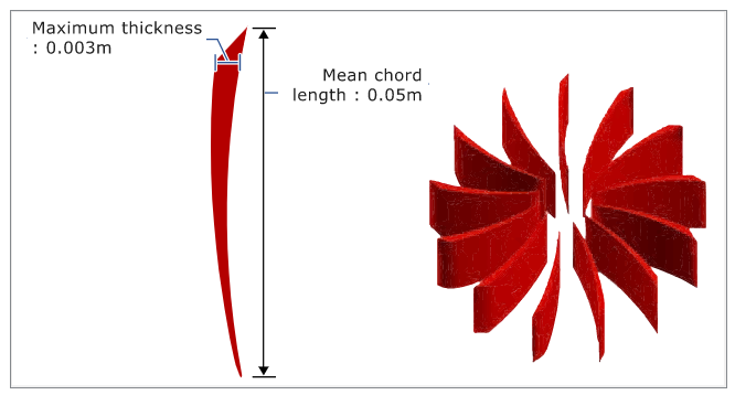
Figure 2. Schematic of Fan Blades
Open the HyperMesh Model Database
-
Click the Open Model icon
 located on the standard toolbar.
The Open Model dialog opens.
located on the standard toolbar.
The Open Model dialog opens.
Set the General Simulation Parameters
In this step, you will set the simulation parameters that apply globally to the simulation.
-
Change the Turbulence model to Spalart Allmaras.
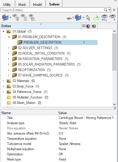
Figure 3.
Create a Moving Reference Frame
In this step, you will create a rotating reference frame for the fluid in the impeller region so that the elements in those regions are solved in the given rotating reference frame and rotational body forces are added to that volume set.
-
Set the Angular velocity-Z to -157.08 rad/sec.
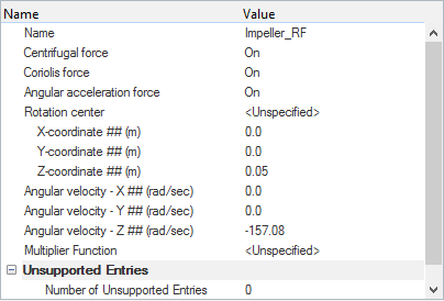
Figure 4.
Set Up Boundary Conditions and Material Model Parameters
-
Click Inlet. In the Entity Editor,
- Change the Type to INFLOW.
- Set the Inflow type to Stagnation Pressure.
- Set the Turbulence input type to Viscosity Ratio.
- Set the Material to Air_HM.
- Set the Turbulence viscosity ratio to 10.0.
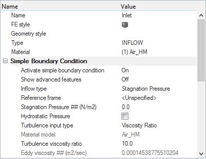
Figure 5. -
Click Outlet. In the Entity Editor, change the Type to OUTFLOW.
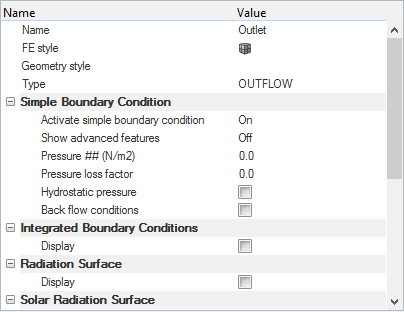
Figure 6. -
Click Walls. In the Entity Editor, verify that the Type is set to WALL.
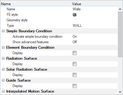
Figure 7.All the surface elements that make up the outer wall of the blower, the fan blades and the interface between the impeller and main fluid can be grouped into one surface set. Auto_Wall, which is an advanced feature in AcuSolve, re-groups these elements into external and internal walls and applies appropriate wall and interface conditions. In this case, the surface elements on the fan blades are grouped together (AUTO Fluid_Impeller wall) and the reference frame assigned to the impeller fluid will be inherited. The surface elements on the interface will be grouped into (AUTO Fluid_Impeller internal) and the elements on the outer casing will be grouped into (AUTO Fluid_Main wall). This entire process of grouping is done internally without you having to do it manually
-
Click Fluid_Main. In the Entity Editor,
- Change the Type to FLUID.
- Select Air_HM as the Material.
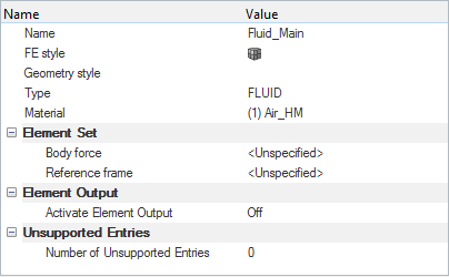
Figure 8. -
Click Fluid_Impeller. In the Entity Editor,
- Change the Type to FLUID.
- Select Air_HM as the Material.
- Select Impeller_RF as the Reference frame.
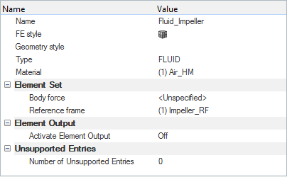
Figure 9.
Compute the Solution
In this step, you will launch AcuSolve directly from HyperMesh and compute the solution.
Run AcuSolve
-
Click
 on the ACU toolbar.
The Solver job Launcher dialog opens.
on the ACU toolbar.
The Solver job Launcher dialog opens. -
Leave the remaining options as
default and click Launch to start the solution
process.
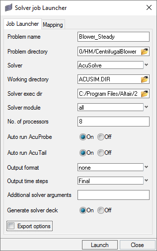
Figure 10.
Post-Process the Results
Create a Pressure-Rise Plot in AcuProbe
As the solution progresses, the AcuTail and AcuProbe windows are launched automatically. In this step, you will create a User Defined Function (UDF) and generate a plot of the pressure rise between the inlet and outlet.
-
Once the solution has converged, click the User Function icon
 in the AcuProbe
window.
A User Function dialog opens.
in the AcuProbe
window.
A User Function dialog opens. -
On the next line, type value = P_Outlet - P_Inlet.
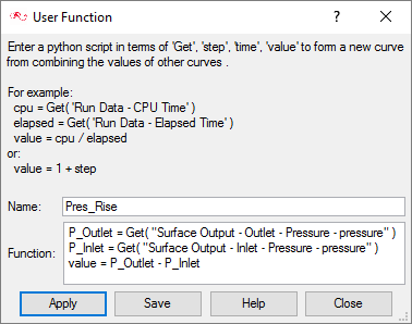
Figure 11.Note: The word “value” is case sensitive and should always be in lowercase characters. If it starts with a capital letter, it will give you an error window. -
Click Apply to display the plot.
Note: You might need to click
 on the toolbar in order to
properly display the plot.
on the toolbar in order to
properly display the plot.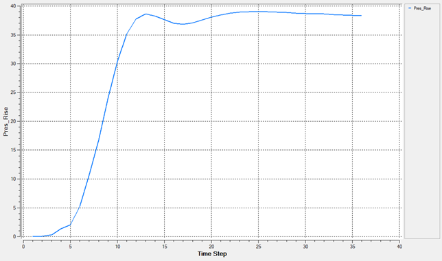
Figure 12.
Open HyperView and Load the Model and Results
-
In the Load model and results panel, click
 next
to Load model.
next
to Load model.
Create a Pressure Contour on a Section Cut Plane
-
Click
 on the Results toolbar to open the Contour panel.
-
In the panel area, under the Display tab, turn off
the Discrete color option.
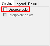
Figure 13. -
Adjust the orientation in the graphics window for a better view of the results
and verify that the contour plot looks like the figure below.
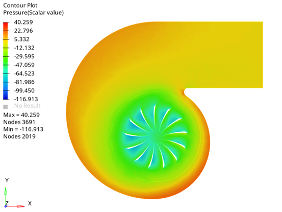
Figure 14.
Summary
In this tutorial, you successfully learned how to set up a steady state simulation involving a rotating reference frame in a centrifugal blower. You started by importing the mesh and then once the case was set up, you generated a solution using AcuSolve. Then, you computed the pressure rise using AcuProbe and created a contour plot for pressure on a cut plane using HyperView.