This tutorial provides the instructions for setting up, solving and viewing results for a
steady simulation of a centrifugal air blower utilizing reference frames. In this
simulation, AcuSolve is used to compute the motion of fluid due to the
rotation of the impeller blades as well as the resulting pressure drop created between the
inlet and outlet after the blades have been rotating for a long time. This tutorial is
designed to introduce you to a number of modelling concepts necessary to perform simulations
that use multiple reference frames.
The basic steps in any CFD simulation are shown in ACU-T: 2000 Turbulent Flow in a Mixing Elbow. The following additional
capabilities of AcuSolve are introduced in this
tutorial:
Rotating reference frame
Assigning of reference frame to volume and surface sets
Post-processing using user function with AcuProbe
Post-processing the nodal output with AcuFieldView to get
pressure fields.
Prerequisites
You should have already run through the introductory tutorial, ACU-T: 2000 Turbulent Flow in a Mixing Elbow. It is assumed that you have some
familiarity with AcuConsole, AcuSolve, and AcuFieldView. You will
also need access to a licensed version of AcuSolve.
Prior to running through this tutorial, copy
AcuConsole_tutorial_inputs.zip from
<Altair_installation_directory>\hwcfdsolvers\acusolve\win64\model_files\tutorials\AcuSolve
to a local directory. ExtractCentrifugal_Blower.x_tfrom AcuConsole_tutorial_inputs.zip.
Analyze the Problem
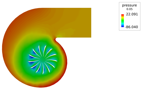
The problem to be addressed in this tutorial is shown schematically in Figure 1 and Figure 2. It consists of a centrifugal
blower with a wheel of forward curved blades, and a housing with inlet and outlet ducts. The
fluid through the inlet plane enters the hub of the blade wheel, radially accelerates due to
centrifugal force as it flows over the blades, and then exits the blower housing through the
outlet plane. Because they're relatively cheaper and simpler than axial fans, centrifugal blowers
have been widely used in HVAC (heating, ventilating, and air conditioning) systems of buildings.
The diameter of the inlet plane is 0.1 m and the length of the inlet duct is 0.15 m. The
housing width is 0.1 m and the radius of the housing from the blade wheel hub varies from 0.113
to 0.18 m. Figure 1. Schematic of Centrifugal Blower
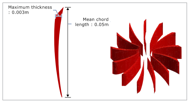
The fan blades have a mean chord length and width of 0.05 m. The maximum thickness of the
blades is 0.003 m. The fan blades have an angular velocity of -1500 RPM. The negative sign
describes the direction of the angular velocity vector which in this case is in the –Z direction
(clockwise rotation). Figure 2. Schematic of Fan Blades
The boundary condition at the inlet is taken as stagnation pressure rather than mass flow rate
so that AcuSolve calculates mass flow rates and pressure rise based
on impeller rotation.
The fluid in this problem is air, which has a density (ρ) of 1.225 kg/m3 and a
viscosity (μ) of 1.781 X 10⁻⁵ kg/m-sec.
In addition to setting appropriate conditions for the simulation, it is important to generate a
mesh that will be sufficiently refined to provide good results. For this problem the global mesh
size is set to provide approximately 16 elements around the circumference of the inlet which
results in a mesh size of 0.02 m. Note that higher mesh densities are required where velocity,
pressure and eddy viscosity gradients are larger. In this application, the flow will accelerate
as it passes through radial flow paths between the fan blades. This leads to the higher gradients
that need finer mesh resolution. Proper boundary layer parameters need to be set to keep the y+
near the wall surface to a reasonable level. The mesh density used in this tutorial is coarse and
is intended to illustrate the process of setting up the model and to retain a reasonable run
time. A significantly higher mesh density is needed to achieve a grid converged solution.
Once a solution is calculated, the flow properties of interest are the mass flow rate at the
outlet and the pressure drop across the inlet and outlet. These parameters define the performance
characteristics.
Define the Simulation Parameters
Start AcuConsole and Create the Simulation Database
In this tutorial, you will begin by creating a database, populating the
geometry-independent settings, loading the geometry, creating groups, setting group
parameters, adding geometry components to groups, and assigning mesh controls and
boundary conditions to the groups. Next you will generate a mesh and run AcuSolve to compute the steady state solution. Finally, you will
visualize the results using AcuFieldView.
In the next steps you will start AcuConsole, and create
the database for storage of the simulation settings.
Start AcuConsole from the Windows Start menu by clicking Start > Altair <version> > AcuConsole.
Click the File menu, then click
New to open the New data
base dialog.
Browse to the location that you would like to use as your working
directory.
This directory is where all files related to the simulation will
be stored. The AcuConsole database file
(.acs) is stored in
this directory. Once the mesh and solution are created, additional files and
directories will be created within this directory.
Create a new directory in this location. Name it
Blower_MRF_Steady and open it.
Enter Blower_MRF_Steady as the file name for the
database.
Note: In order for other applications to be able to read the
files written by AcuConsole, the database
path and name should not include spaces.
Click Save to create the database.
Set General Simulation Parameters
In next steps you will set parameters that apply globally to
the simulation. To make this simple, the basic settings applicable for any
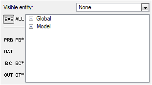
simulation can be filtered using the BAS filter in the Data Tree Manager. This filter enables display of only a small subset
of the available items in the Data Tree and makes navigation
of the entries easier.
The physical models that you define for this tutorial correspond to steady state,
turbulent flow.
Click BAS in the Data Tree Manager to switch to basic view in the Data Tree.
Figure 3.
Double-click the GlobalData Tree item to expand it.
Tip: You can also expand a tree item
by clicking
next to the item name. Figure 4.
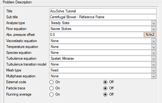
Double-click Problem
Description to open the Problem
Description detail panel.
Tip: You can also open a panel by right-clicking a tree item and
clicking Open on the context menu.
Enter AcuSolve Tutorial as the Title.
Enter Centrifugal Blower - Reference Frame as the Sub
title.
Accept the default Analysis type as Steady State.
Change the Turbulence equation to Spalart
Allmaras.
Accept the default Mesh type of Fixed.
Figure 5.
Set Solution Strategy Parameters
In the next steps you will set parameters that control the behavior of AcuSolve as it progresses during the solution.
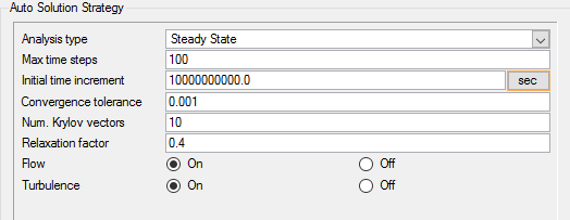
Double-click Auto Solution
Strategy to open the Auto Solution
Strategy detail panel.
Check that the Analysis type is set to Steady State.
Set the Max time steps as 100.
Check that the Convergence tolerance is set to 0.001.
Set the Relaxation factor to 0.4.
The relaxation factor is used to improve convergence of the solution.
Typically, a value between 0.2 and 0.4 provides a good balance between achieving
a smooth progression of the solution and the extra compute time needed to reach
convergence. Higher relaxation factors cause AcuSolve to take more time steps to reach a steady state solution. A high relaxation
factor is sometimes necessary in order to achieve convergence for very complex
applications. Figure 6.
Set Material Model Parameters
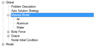
AcuConsole has three pre-defined materials, Air,
Aluminum, and Water, with standard parameters defined. In the next steps you will verify
that the pre-defined material properties of air match the desired properties for this
problem.
Double-click Material Model
in the Data Tree to expand it.
Figure 7.
Double-click Air in the
Data Tree to open the Air
detail panel.
The material type for air is Fluid. Fluid is
the default material type for any new material created in AcuConsole.
Click the Density tab. The density of air is 1.225
kg/m3.
Click the Viscosity tab. The viscosity of air is 1.781 x
10-5kg/m – sec.
Save the database to create a backup
of your settings. This can be achieved with any of the following
methods.
Click the File menu, then click
Save.
Click on
the toolbar.
Click Ctrl+S.
Note: Changes made in AcuConsole are saved into
the database file (.acs) as they are made. A save operation copies the database to
a backup file, which can be used to reload the database from that saved
state in the event that you do not want to commit future changes.
Import the Geometry and Define the Model
Import the Geometry
You will import the geometry in the next
part of this tutorial. You will need to know the location ofCentrifugal_Blower.x_tin order to complete these steps. This file contains
information about the geometry in ParasolidASCII format.
Click File > Import.
Browse to the directory containing Centrifugal_Blower.x_t.
Change the file name filter to Parasolid File (*.x_t *.xmt *X_T
…).
Select Centrifugal_Blower.x_t and click
Open to open the Import Geometry
dialog.
Figure 8.
For this tutorial, the default values for the Import
Geometry dialog are used to load the geometry. If you have previously
used AcuConsole, be sure that any settings that you
might have altered are manually changed to match the default values shown in the
figure. With the default settings, volumes from the CAD model are added to a default
volume group. Surfaces from the CAD model are added to a default surface group. You
will work with groups later in this tutorial to create new groups, set flow
parameters, add geometric components, and set meshing parameters.
Click Ok to complete
the geometry import.
Figure 9.
The color of objects shown in the modeling window in this tutorial and those displayed on your screen may differ. The default color
scheme in AcuConsole is "random," in which colors are
randomly assigned to groups as they are created. In addition, this tutorial was
developed on Windows. If you are running this tutorial on a different operating system,
you may notice a slight difference between the images displayed on your screen and the
images shown in the tutorial.
Create a Reference Frame
A reference frame is used to specify a rotating frame of reference. When specified
for a volume set in domain, the elements in that volume set are assumed to be solved
in the given rotating reference frame and rotational body forces are added for that
volume set. In this tutorial, the fluid region near the impeller blades is assigned
a rotating reference frame.
In the next steps you will create a reference frame.
Click PB* in the Data Tree Manager to display all the available settings related to general problem setup in
the Data Tree.
Expand the GlobalData Tree item.
Right-click Reference Frame and click New
to create a new reference frame.
Rename the new reference frame.
Right-click Reference Frame 1.
Click Rename.
Type Impeller_RF and press Enter.
Double-click Impeller_RF to open the detail panel.
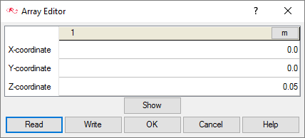
Click the Open Array button next to Rotation center to
open the Array Editor.
Enter 0.05 as the Z-coordinate.
Figure 10.
Click OK to close the dialog.
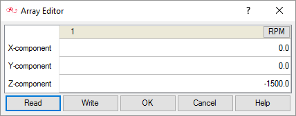
In the detail panel, click the Open Array button next to
Angular velocity to open the Array Editor.
Change the units to RPM and enter
-1500 in the Z-component field.
Note: The negative sign specifies the clockwise direction of rotation. Note that
the rotation direction is determined using the “right-hand rule”.
Figure 11.
Click OK to close the dialog.
Apply Volume Parameters
Volume groups are containers used for storing information about a volume region. This
information includes the list of geometric volumes associated with the container, as
well as attributes such as material models and mesh size information.
When the geometry was imported into AcuConsole, all
volumes were placed into the "default" volume container.
In the next steps you will create a new volume group, assign a volume to that group,
rename the default volume group container, assign the materials for the groups, and
set the reference frame for the impeller volume.
Click BAS in the Data Tree Manager to switch to basic view in the Data Tree.
Expand the ModelData Tree item.
Expand Volumes. Toggle the display of the default
volume container by clicking
and next to the volume name.
Note: You may not see any change when toggling the display if
Surfaces are being displayed, as surfaces and
volumes may overlap.
Create a new volume group.
Right-click on Volumes.
Click New.
Rename the new volume group to Fluid_main.
Add the fluid volume to the Fluid_main volume group.
Right-click on the Fluid_main volume
group.
Click Add to and select the volume to add it to
the volume group.
The fluid main volume should now be highlighted in a grey color. Figure 12.
When the geometry was loaded into AcuConsole,
all geometry volumes were placed in the default volume group container. At this
point, all the remaining volumes are in the default volume group. Rather than create
a new container, add the flow volume in the geometry to it, and then delete the
default volume container, you will rename the container and modify the parameters
for this group.
Rename the default volume group to Fluid_Impeller.
Check that the material model for the volumes is set as Air.
Double click Element Set under Fluid_Main to
open it in the detail panel.
Ensure that the Material model is set to Air.
Assign the reference frame Impeller_RF to
Fluid_Impeller.
Figure 13.
Create Surface Groups and Apply Surface Boundary
Conditions
Surface groups are containers used for storing information
about a surface or a set of surfaces. This information includes the list of
geometric surfaces associated with the container, as well as attributes such as
boundary conditions, surface outputs and mesh sizing information.
In the next steps you will define surface groups, assign the appropriate settings for
the different characteristics of the problem and add surfaces to the group
containers.
Inlet
Outlet
Walls
Interface
Fan Blades
Set Parameters for the Inlet
In the next steps you will define a surface group for the
inlet, assign the appropriate settings, and add the inlet from the geometry to the
surface group.
Collapse Volumes in the Data Tree.
Create a new surface group.
Rename the new surface to Inlet.
Expand Inlet in the Data Tree.
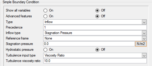
Double-click Simple Boundary Condition to open the
detail panel.
Change the Type to Inflow.
Change the Inflow type to Stagnation Pressure.
Change the Turbulent input type to Viscosity Ratio.
This allows you to automatically compute the eddy viscosity value based on the
material model and the ratio of the turbulent to molecular viscosity.
Set the Turbulence viscosity ratio to 10.
Figure 14.
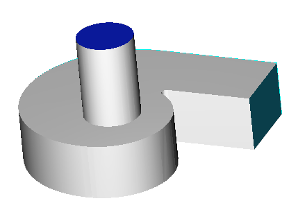
Add geometry to the Inlet group.
In the tree, right-click on Inlet and select
Add to.
Click on the inlet face on the model.
At this point, the inlet should be highlighted grey. Figure 15.
Click Done to add this geometry surface to the
Inlet surface group.
Tip: You can also use the middle mouse button to complete
the addition of geometry components to a group.
Set Parameters for the Outlet
In the next steps you will define a surface group for the
outlet, assign the appropriate settings, and add the outlet from the geometry to the
surface group.
Create a new surface group.
Rename the new surface to Outlet.
Expand Outlet in the Data Tree.
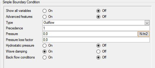
Double-click Simple Boundary Condition to open the
detail panel.
Change the Type to Outflow.
Figure 16.
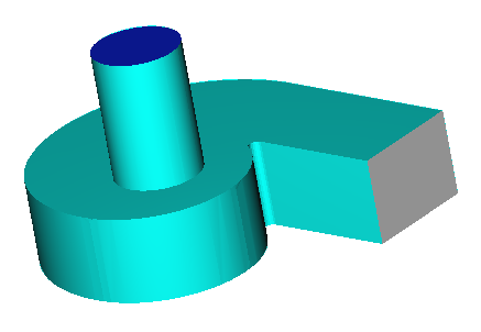
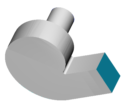
Add geometry to the Outlet surface container.
In the tree, right-click on Outlet and select
Add to.
Click on the outlet face on the model.
At this point, the outlet should be highlighted grey. Figure 17.
Click Done to add this geometry surface to the
Outlet surface group.
Set Parameters for the Walls
In the next steps you will define a surface group for the
walls, assign the appropriate settings, and add the faces from the geometry to the
surface group.
Create a new surface group.
Rename the new surface to Walls.
Expand Walls in the Data Tree.
Double-click Simple Boundary Condition to open the
detail panel.
Check that the Type is set to Wall.
Add geometric faces to the Wall group.
In the tree, right-click on Walls and select
Add to.
Select all the wall surfaces.
At this point, the wall surfaces should be highlighted grey.
Figure 18. Figure 19.
Click Done to associate this geometry surface
with the Walls surface container.
Set Parameters for the Interface
In the next steps you will define a surface group for the
Interface, assign the appropriate settings, and add the Interface surfaces from the
geometry to the surface group.
Note: Internal surfaces in AcuConsole are handled in a special manner. At import
time, AcuConsole creates two identical copies of the
surface. One copy of the surface is associated with each volume. This allows you
to control meshing parameters independently on each side of the surface. When
assigning boundary conditions to internal surfaces, it is important to remember
that there are two sides of the surface that need to be dealt with. When
selecting an internal surface, the side corresponding to the outer volume is the
first pick target that is encountered when both faces are visible. The inner
surface can be selected directly by changing the display of the outer
surface.
Turn off the display of the Inlet, Outlet, and Walls surfaces.
Create a new surface group.
Rename the new surface to Interface.
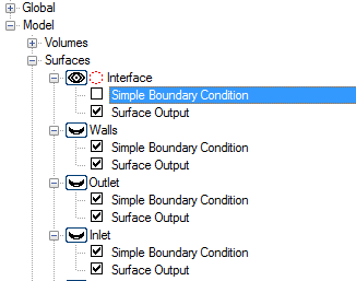
Expand Interface in the Data Tree.
Turn off the Simple Boundary Condition by unchecking the box next to it.
Figure 20.
Add geometry surfaces Interface group.
In the tree, right-click on Interface and
select Add to.
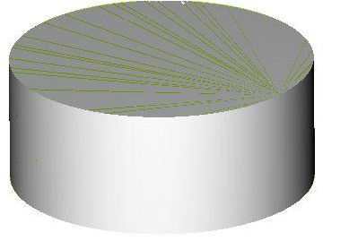
Select all the surfaces on the interface.
Click Done to associate this geometry surface
with the Walls surface container.
Figure 21.
Turn off the display for the interface.
There are two sets of surfaces for the interface which belong to different
volume sets. In this case they can be moved into the same surface
group.
Right-click Interface and click Add
to.
Select the remaining interface surfaces.
Click Done to associate this geometry surface with the
surface settings of the Interface group.
Note: Note that no boundary conditions are applied to this surface at this
point. The grouping operation was performed to identify that these surfaces
are internal and that flow will be allowed to pass through them freely.
These surfaces can still be used for output purposes, however.
Set Parameters for the Fan Blades
In the next steps you will define a surface group for the
Fan_Blades, assign the appropriate settings, and add the fan blades from the
geometry to the surface group.
Rename the default surface to Fan_Blades.
Expand Fan_Blades in the Data Tree.
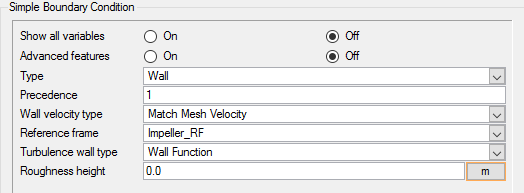
Double-click Simple Boundary Condition to open the
detail panel.
The default Type for a default surface is Wall.
Set the Reference frame as Impeller_RF.
Figure 22.
Assign Mesh Controls
Set Global Mesh Parameters
Now that the flow characteristics have been set for the whole problem and for the
individual surfaces, attributes need to be added to make sure that a sufficiently
refined mesh is generated.
Global mesh controls apply to the whole model without being tied to any
geometric component of the model.
Zone mesh controls apply to a defined region of the model, but are not
associated with a particular geometric component.
Geometric mesh controls are applied to a specific geometric component. These
controls can be applied to volume groups, surface groups, or edge
groups
In the next steps you will set the global mesh attributes. In subsequent steps you
will set the surface meshing attributes.
Click MSH in the Data Tree Manager to filter the
settings in the Data Tree to show only the controls
related to meshing.
Double-click the GlobalData Tree item to expand it.
Double-click Global Mesh
Attributes to open the Global Mesh
Attributes detail panel.
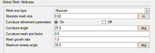
Change the Mesh size type to Absolute.
Enter 0.02 m for the Absolute mesh size.
This absolute mesh size is chosen to ensure that there are at least 50 mesh
elements on the inlet.
Set the Maximum sweep angle as 30.0 degrees.
This option allows you to set the maximum sweep angle for edge blend meshing
on a global basis which creates a radial array of elements around sharp edges to
provide better resolution of the flow features. The sweep angle is used to
control how many degrees each radial division spans. Figure 23.
Set Surface Mesh Parameters
In the following steps you will set the meshing attributes that will allow for
localized control of the mesh size on the surface groups that you created earlier.
Specifically, you will set local meshing attributes that control the growth of
boundary layer elements normal to the surfaces of the walls and fan blades.
Walls
Fan Blades
Set Surface Mesh Parameters for the Walls
In the following steps you will set meshing attributes that will allow for localized
control of the mesh size near the walls. The mesh size on the wall will be inherited
from the global mesh size that was defined earlier. The settings that follow will
only control the growth of the boundary layer from the walls.
Expand the ModelData Tree item.
Under the Model branch, expand Surfaces, and then expand
Walls.
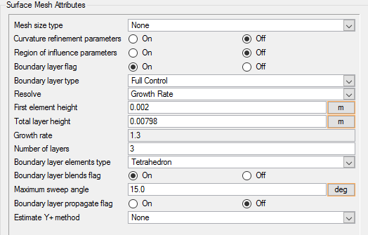
Click the check box next to Surface Mesh Attributes to enable the settings and
open the Surface Mesh Attributes detail panel.
Change the Mesh size type to None.
This option indicates that the mesher will use the global meshing attributes
when creating the mesh on the surface of the walls.
Switch the Boundary layer flag to On.
This option allows you to define how the meshing should be handled in
the direction normal to the walls.
Set the Boundary layer type to Full Control.
Mesh elements for a boundary layer are grown in the normal direction from a
surface to allow efficient resolution of the steep gradients near no-slip walls.
The layers can be specified using a number of different options.
When
Boundary layer type is set to Full Control, the First layer height, Number
of layers and the Growth rate are specified. Boundary layer elements will be
grown until the mesh size of the top layer matches the mesh size of the
volume into which the boundary layer elements are grown.
Set the remaining settings as follows:
Option
Description
First element height
0.002
Number of layers
3
Boundary layer bends flag
On
Maximum sweep angle
15.0
Figure 24.
Set Surface Mesh Parameters for the Fan Blades
In the following steps you will set meshing attributes that will allow for localized
control of the mesh size near the fan blades.
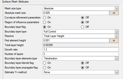
Under Fan Blades, click the check box next to Surface Mesh Attributes to enable
the settings and open the Surface Mesh Attributes detail
panel.
Change the Mesh size type to Absolute.
Enter 0.005 m as the Absolute mesh size.
Switch the Boundary layer flag to On.
Set the Boundary layer type to Full Control.
Set the Resolve field to Total Layer Height.
Set the remaining settings as follows:
Option
Description
First element height
0.001 m
Growth rate
1.3
Number of layers
3
Figure 25.
Save the database to create a backup of your settings.
Generate the Mesh
In the next steps you will generate the mesh that will be used when computing a
solution for the problem.
Click on the toolbar to open the Launch
AcuMeshSim dialog.
Click Ok to begin meshing.
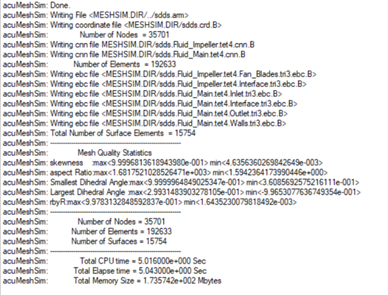
During meshing an AcuTail window opens. Meshing
progress is reported in this window. A summary of the meshing process indicates that the
mesh has been generated.
Figure 26.
Note: The actual number of nodes and elements, and memory usage may vary
slightly from machine to machine.
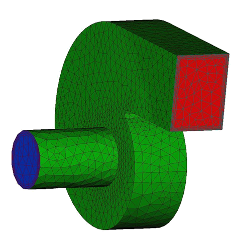
Visualize the mesh in the modeling window. For the
purposes of this tutorial, the following steps lead to the display of inlet,
outlet, walls and fan blades.
Right-click Volumes in the Data Tree and click Display off.
Right-click Surfaces in the Data Tree and click Display on.
Right-click Surfaces in the Data Tree, select Display type and
click solid & wire.
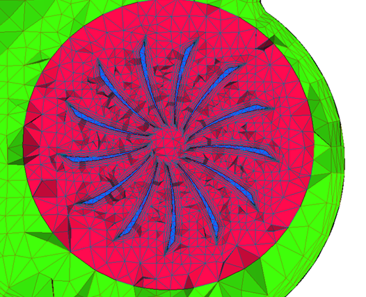
Rotate and zoom in the model to analyze the various mesh regions.
Right-click on the model and select cut plane
visualization to view the mesh near the fan blades.
Figure 27. Mesh Details of the GeometryFigure 28. Mesh Details Near the Fan Blades
Save the database to create a backup of your settings.
Compute the Solution and Review the Results
Run AcuSolve
In the next steps you will launch AcuSolve to compute the solution for this case.
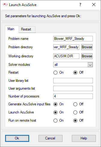
Click on the toolbar to open the
Launch AcuSolve dialog.
Figure 29.
Enter 4 for Number of processors, if your system has 4
or more processors.
The use of multiple processors can reduce solution time.
Accept all other default settings.
Based on these settings, AcuConsole will generate
the AcuSolve input files and then launch the
solver.
Click Ok to start the
solution process.
While computing the solution, an
AcuTail window opens. Solution progress is
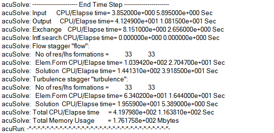
reported in this window. A summary of the solution process indicates
that the run has been completed.
The information provided in the summary is based on
the number of processors used by AcuSolve.
If you use a different number of processors than indicated in this
tutorial, the summary for your run may be slightly different than the
summary shown.
Figure 30.
Close the AcuTail window and save the database to create a
backup of your settings.
Monitor the Solution with AcuProbe
AcuProbe can be used to monitor various variables over
solution time.
Open AcuProbe by clicking on the toolbar.
In the Data Tree on the left, expand
Residual Ratio.
Right-click on Final and select Plot
All.
The residual ratio measures how well the solution matches the governing
equations.
Note: You might need to click on the toolbar in order to
properly display the plot.
Figure 31.
After AcuSolve has finished running, a summary of the
solution process showing the “End Time Step” data indicates that the simulation
has been completed.
Post-Process with AcuProbe
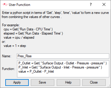
The pressure rise between the Inlet and Outlet can be viewed using a User Function at
the end of simulation using AcuProbe.
In the AcuProbe window, double-click on .
Enter the name in the User Function window as
Pres_Rise.
In the function window, type P_Outlet =.
Expand Surface Output > Outlet > Pressure.
Right-click on pressure and select Copy
Name.
Paste the value in the function window for Outlet pressure.
Type P_Inlet = on a line line.
Repeat steps 4 - 6 for Inlet pressure.
Type value = P_Outlet – P_Inlet.
Figure 32.
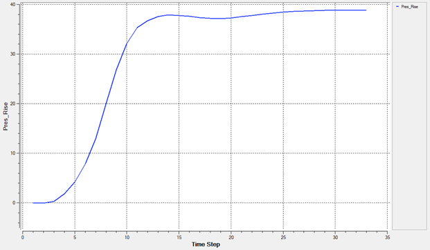
Click Apply to display the plot.
Note: You might need to click on the toolbar in order to
properly display the plot.
Figure 33.
View Results with AcuFieldView
Now that a solution has been calculated, you are ready to view the flow field using AcuFieldView. AcuFieldView is based on a
third-party post-processing tool that has been tightly integrated toAcuSolve. AcuFieldView can be started
directly from AcuConsole, or it can be started from the Start
menu, or from a command line. In this tutorial you will start AcuFieldView from AcuConsole after the
solution is calculated by AcuSolve.
Start AcuFieldView
Click on the
AcuConsole toolbar to open the
Launch AcuFieldView dialog.
Click Ok to start
AcuFieldView.
When you start AcuFieldView from AcuConsole, the results from the last time step of the
solution that were written to disk will be loaded for post-processing.
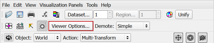
View the Boundary Surface Showing Pressure for the Outer Surfaces with Mesh
Click Viewer Options.
Figure 34.
Click axis markers to disable them.
Uncheck Perspective to disable perspective view.
Close the Viewer Options dialog.
Change the background color to white
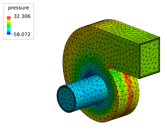
Orient the geometry so you can see inlet, outlet and wall surfaces as shown in
Figure 35.
In the Boundary Surfaces dialog, ensure that
Pressure is selected as the Scalar function.
In the Boundary Types list, select the Inlet,
Outlet and Wall surfaces from
boundary types.
Click on the Colormap tab and check
Local to display the local range of values of
pressure for the selected surfaces.
Add a legend to the view.
In the Boundary Surface dialog, click the
Legend tab.
Enable the Show Legend option.
Enable the Frame option.
In the Color group, next to Geometric, click the white color swatch,
and then select the black color swatch to set the color for the legend
values to black.
Click the white color swatch next to the Title field and set the color
for the title to black.
Move the legend by Shift+left-clicking and
dragging the legend to the left.
Figure 35.
Coordinate the Surface Showing Pressure on the Mid Coordinate Surface
Click to open
the Coordinate Surface dialog.
Click Create to create a new surface.
Set the new surface at the mid –Z coordinate surface.
In the Coord Plane fields, enter
0.05 as the Current value.
This is the z coordinate for the mid plane between the blower front and back
walls.
Change the Display Type to smooth.
Change the Coloring to scalar.
Select pressure as the scalar function to display.
Click the Colormap tab and change the coloring to
local.
Turn on the legend to display the pressure values on the coordinate
plane.
Orient the geometry for a better view of the results.
Figure 36.
Summary
In this tutorial, you worked through a basic workflow to set up a steady state simulation with
a rotating reference frame in a centrifugal blower. Once the case was set up, you generated a
mesh and generated a solution using AcuSolve. AcuProbe was used to post-process the pressure rise in the blower. Results
were also post-processed in AcuFieldView to allow you to create
contour views for the pressure along the walls and on the mid coordinate surface of the blower.
New features introduced in this tutorial include creating a rotating reference frame and creating
a user function in AcuProbe.

 next to the item name.
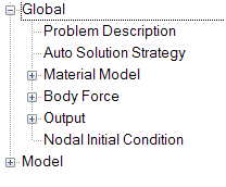
 on
the toolbar.
on
the toolbar.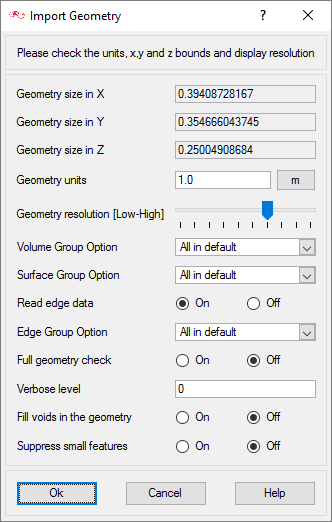

 and
and  next to the volume name.
Note: You may not see any change when toggling the display if Surfaces are being displayed, as surfaces and volumes may overlap.
next to the volume name.
Note: You may not see any change when toggling the display if Surfaces are being displayed, as surfaces and volumes may overlap.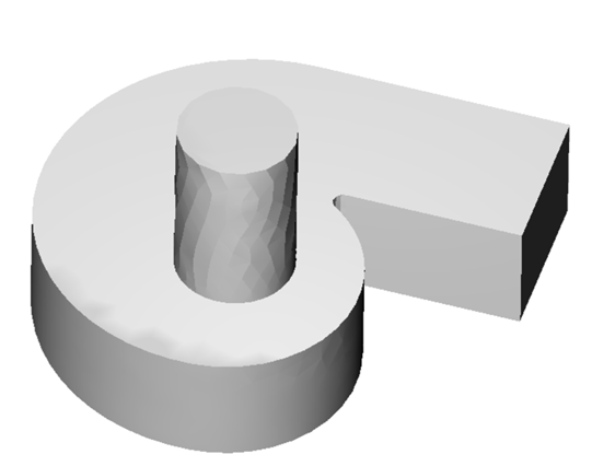


 on the toolbar to open the Launch
AcuMeshSim dialog.
on the toolbar to open the Launch
AcuMeshSim dialog.
 on the toolbar to open the
Launch AcuSolve dialog.
on the toolbar to open the
Launch AcuSolve dialog.
 on the toolbar.
 on the toolbar in order to
properly display the plot.
on the toolbar in order to
properly display the plot.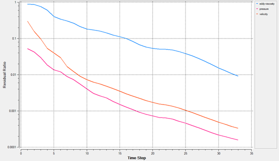
 .
.
 on the
AcuConsole toolbar to open the
Launch AcuFieldView dialog.
on the
AcuConsole toolbar to open the
Launch AcuFieldView dialog.
 to open
the Coordinate Surface dialog.
to open
the Coordinate Surface dialog.