SOLAR_RADIATION
Specifies global solar radiation algorithms and parameters.
Type
AcuSolve Command
Syntax
SOLAR_RADIATION {parameters}
Qualifier
This command has no qualifier.
Parameters
- type (enumerated) [=piecewise_linear]
- Type of solar heat flux.
- piecewise_linear or linear
- Piecewise linear curve fit. Requires curve_fit_values and curve_fit_variable.
- curve_fit_values or curve_values (array) [={0,0,0,-1352}]
- A four-column array of independent-variable/solar-flux-vector data values. Used with piecewise_linear type.
- curve_fit_variable or curve_var (enumerated) [=time]
- Independent variable of the curve fit. Used with piecewise_linear type.
- time
- Current run time.
- multiplier_function (string) [=none]
- User-given name of the multiplier function for scaling the solar flux vector. If none, no scaling is performed.
- computation_type (enumerated) [=ray_trace]
- Type of algorithm used to compute the solar heat flux
- ray_trace
- Ray trace algorithm. Requires num_rays, num_diffuse_sub_rays max_ray_reflections, min_ray_energy and terminated_ray_redistribution_factor
- num_rays (integer) >=1 [=1000000]
- Number of rays for the solar heat flux calculation. Used with ray_trace computational type.
- num_diffuse_sub_rays (integer) >=1 [=4]
- Number of sub-rays a ray is split into for diffuse reflections and transmissions. Used with ray_trace computational type.
- max_ray_reflections (integer) >=0 [=10]
- Maximum number of times a single ray is allowed to reflect before it is terminated. Used with ray_trace computational type.
- min_ray_energy (real) >=0 [=1.e-3]
- Minimum relative energy a ray is allowed to have before it is terminated. Used with ray_trace computational type.
- terminated_ray_redistribution_factor (real) >=0 <=1.0 [=1.0]
- Factor for distributing the remaining energy of a terminated ray. Used with ray_trace computational type.
- smoothing or smooth (boolean) [=on]
- Flag specifying whether to spatially smooth the solar heat flux.
Description
This command specifies the global parameters for solar radiation heat flux as defined by the SOLAR_RADIATION_SURFACE and SOLAR_RADIATION_MODEL commands. These parameters do not apply to radiation boundary conditions defined by ELEMENT_BOUNDARY_CONDITION commands or to RADIATION or related commands.
SOLAR_RADIATION {
   type                                    = piecewise_linear
   curve_fit_values                        = { 0, 0, 0, -1352 }
   curve_fit_variable                      = time
   computation_type                        = ray_trace
   num_rays                                = 1000000
   num_diffuse_sub_rays                    = 4
   max_ray_reflections                     = 10
   min_ray_energy                          = 1.e-3
   terminated_ray_redistribution_factor    = 1
   smoothing                               = on
}
specifies that the solar radiation heat fluxes are to be added to the thermal energy equation based on a constant solar flux of 1352 in the negative z direction. The fluxes are to be computed using a ray trace algorithm with 1000000 initial rays, diffuse reflections and transmissions split into 4 sub-rays, a maximum of 10 reflections and a minimum relative energy of  before a ray is terminated, and the remaining energy of a terminated ray distributed over the previous absorptions of this ray. The computed solar heat flux is then spatially smoothed.
Local Surface Coordinate System
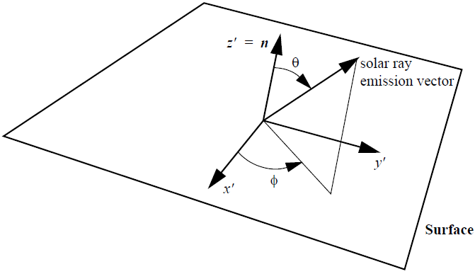
Figure 1.
where is the specular transmissivity, is the diffuse transmissivity, is the specular reflectivity, is the diffuse reflectivity and is the absorptivity, The transmissivity and reflectivity properties are defined by the SOLAR_RADIATION_MODEL command, and the absorptivity by the above constraint. The energy distribution of a diffuse reflection or transmission must be proportional to cos( ) in order to obtain a uniform distribution of outgoing energy over the projected surface area.
The type, curve_fit_values, and curve_fit_variable parameters define the global incoming solar flux vector. A linear_curve_fit type interpolates the data in curve_fit_values linearly. The first column in this array is curve_fit_variable, and the second, third, and fourth are the three components of the global solar heat flux vector. The default of (0,0,-1352) is in W/m2, and is a typical value. The independent variable values must be in ascending order. The limit point values of the curve fit are used when curve_fit_variable falls outside of the curve fit limits. Thus for a constant solar heat flux, just one line in curve_fit_values is needed, as in the example above.
Photon-Surface Interactions
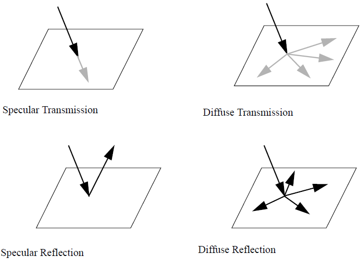
Figure 2.
0        100         200            -1000
1000      80         160            -800
2000 60 120 -600SOLAR_RADIATION {
type = piecewise_linear
curve_fit_values = Read( "solar_heat_flux.dat" )
curve_fit_variable = time
...
}SOLAR_RADIATION {
type = piecewise_linear
curve_fit_values = { 0, 100, 200, -1000 }
curve_fit_variable = time
multiplier_function = "time varying"
...
}
MULTIPLIER_FUNCTION( "time varying" ) {
type = piecewise_linear
curve_fit_values = { 0, 1.0 ;
1000, 0.8 ;
2000, 0.6; }
curve_fit_variable = time
}A ray_trace computational type uses the Monte Carlo method to compute exchange factors and the solar heat flux on every surface specified by the SOLAR_RADIATION_SURFACE commands. This is done as a pre-processing step for every line in curve_fit_values. The heat fluxes are then interpolated during the simulation according to type and curve_fit_variable. Note that if only the magnitude of the solar heat flux vector changes and not the direction, it is less expensive to use the multiplier_function parameter as above.
The first step in the ray_trace computational type is to spread num_rays rays over a rectangle normal to the solar heat flux vector that encompasses all the solar radiation surfaces if they are projected along this vector onto the plane of the rectangle. The cost of the algorithm is proportional to num_rays, so you should be careful with using more rays than the default.
For diffuse transmissions and reflections the uniform distribution of the outgoing energy is approximated by num_diffuse_sub_rays discrete photons. These photons have random energies with the constraint of adding up to the given total energy. Their directions are also random (within the appropriate hemisphere) with a cos( ) probability distribution. The cost of the algorithm can be proportional to as much as the square of this parameter.
Each ray and sub-ray is followed until one of three things happen. First, the ray may not hit any solar radiation surface. In this case its energy does not contribute to the heat flux of any surface. Second, it undergoes max_ray_reflections reflections and is terminated. Third, its relative energy is reduced through absorptions until it reaches min_ray_energy and is terminated. In the last two cases where the ray is terminated the disposal of the remaining energy is determined by terminated_ray_redistribution_factor. A value of zero means that this energy is thrown away and does not contribute to the heat flux of any surface. A value of one means that this energy is to be distributed over the previous surfaces that this ray encountered according to the absorptivity of each surfaces. Values between zero and one interpolate between these two limits.
For some problems a spatially noisy distribution of the solar heat flux results from not using a sufficient number of rays. If increasing the number of rays is too expensive then turning on the smoothing parameter will smooth the solar heat flux while conserving the integrated solar heat flux.