RADIATION
Specifies global radiation algorithms and parameters.
Type
AcuSolve Command
Syntax
RADIATION {parameters}
Qualifier
This command has no qualifier.
Parameters
- view_factor_type (enumerated) [=hemicube]
- Calculation method for the view factor.
- hemicube
- Hemicube. Requires num_hemicube_bins and max_surface_subdivision.
- num_hemicube_bins or bins (integer) >0 [=200]
- Number of bins for the view factor calculation. Used with hemicube view factor type.
- max_surface_subdivision (integer) >=1 [=1]
- Maximum number of segments to split a surface facet when proximity condition is violated. Used with hemicube view factor type.
- smoothing_type (enumerated) [=least_squares]
- Type of view factor smoothing algorithm.
- least_squares
- Least squares smoothing.
- stefan_boltzmann_constant (real) >0 [=5.67e-8]
- Stefan-Boltzmann constant. Default is in MKS units.
- num_symmetry_planes (integer) >=0 <=3 [=0]
- Number of orthogonal symmetry planes in geometrical model.
- symmetry_center or center (array) [={0,0,0}]
- Any point that lies at the intersection of all symmetry planes. Used with num_symmetry_planes>0.
- symmetry_direction_1 (array) [={1,0,0}]
- Normal direction to first symmetry plane. Used with num_symmetry_planes>0.
- symmetry_direction_2 (array) [={0,1,0}]
- Normal direction to second symmetry plane. Used with num_symmetry_planes>1.
- symmetry_direction_3 (array) [={0,0,1}]
- Normal direction to third symmetry plane. Used with num_symmetry_planes=3.
Description
This command specifies the global parameters for enclosure radiation heat transfer as defined by the RADIATION_SURFACE and EMISSIVITY_MODEL commands. Radiation commands with default values are automatically created for the P1 radiation method to model radiative heat transfer in a grey, optically thick participating medium. These parameters do not apply to radiation boundary conditions defined by ELEMENT_BOUNDARY_CONDITION commands or to heat fluxes defined by SOLAR_RADIATION and related commands.
EQUATION {
   ...
   radiation                        = enclosure
   absolute_temperature_offset      = 273.14
}
RADIATION {
   view_factor_type                 = hemicube
   num_hemicube_bins                = 200
   max_surface_subdivision          = 4
   smoothing_type                   = least_squares
   stefan_boltzmann_constant        = 5.67e-08
   num_symmetry_planes              = 1
   symmetry_center                  = { 0, 0, 0 }
   symmetry_direction_1             = { 1, 0, 0 }
}
specifies that the enclosure radiation equation is to be solved, the hemicube algorithm with 200 bins per side is used to calculate the view factor, each radiation facet may be split into a maximum of 4 sub-surfaces to reduce proximity and visibility errors, the least squares method is used to smooth the view factor, the Stefan-Boltzmann constant is 5.67x10-, and one symmetry plane is modeled.
where is the absorptivity and is the reflectivity. From Kirchhoff' law and the grey surface assumption, . The net radiation heat flux is thus and is added to the temperature equation. The radiation equation solves for all the radiation heat fluxes coupled together with the temperature equation.
where Ai and Aj are the areas of surfaces i and j , respectively; and are the angles between the line connecting to and the normals to surfaces to ; respectively; r is the distance from to ; and is the visibility function, it is equal to one if to see each other, otherwise it is zero.
View Factor Nomenclature
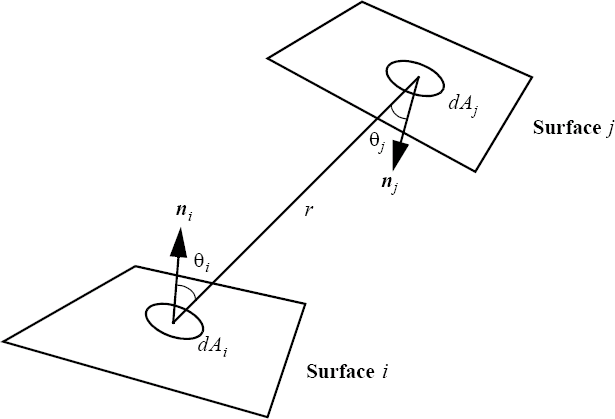
Figure 1.
The view factors are computed using the hemicube algorithm. In a nutshell, in this algorithm a hemicube is placed on the centroid of each radiation facet i. The hemicube is discretized into 3n2 pixels; where n is given by num_hemicube_bins. All surfaces (facing surface i) are then projected onto this hemicube. The Z-buffering algorithm is used to compute the visibility. Once all surfaces are projected, the pixels weighted by their view factor increments are added up to determine a row of Fi={Fij}.
Hemicube Discretization
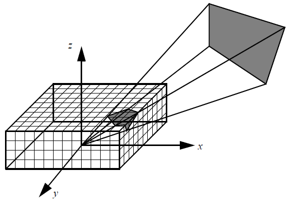
Figure 2.
The hemicube algorithm has three major assumptions, and hence sources of errors: aliasing - the true projection of each visible face onto the hemicube can be accurately accounted for by using a finite resolution hemicube; proximity - the distance between faces is great compared to the effective diameter of the faces; and visibility - the visibility between any two faces does not depend on the position within either face. The aliasing error may be reduced through the use of larger num_hemicube_bins values, at the expense of computational cost. Note that the computational cost is proportional to n2 for sufficiently large values of n. In addition, a random jittering algorithm and a non-uniform hemicube pixelization are employed to minimize the aliasing error. The proximity and visibility errors occur when two facing facets are too close to each other. In this case, the geometry of one or both facets cannot be sufficiently well-represented by their centroids. These errors can be reduced by splitting each poorly-represented facet into smaller segments (sub-surfaces), computing the view factors separately for each sub-surface and then adding them up. The computational cost is proportional to the number of sub-surface divisions. The max_surface_subdivision parameter may be used to trade-off accuracy against cost.
A least-squares smoothing is automatically applied to the computed view factor matrix to enforce reciprocity and conservation:
(reciprocity)
(conservation)
Note that due to the cost of computing the view factor matrix, it is computed in a pre-processing step and stored on disk. This means that the view factors are not updated during a simulation, even when mesh movement is present.
The default for the Stefan-Boltzmann constant is given in MKS units: .
In British units it is: .
In general, this constant must be converted to be consistent with the units chosen for use in the problem.
Symmetry planes may be modeled with num_symmetry_planes>0. This allows geometrical models that are a half, quarter, or eighth of the corresponding "ull"models. All planes must be mutually orthogonal. The radiation facets are reflected across each symmetry plane to create the full model. The view factors are computed on this model before being rescaled to the original model. Note that a given surface facet may then be able to see itself. Normally no RADIATION_SURFACE command is used on a surface lying in any of the symmetry planes, except if (partial) shielding is modeled. Specifying symmetry planes in this command only affects the calculation of view factors and has no effect on any other aspect of the simulation model.