Laminar Flow Through a Pipe with Constant Wall Temperature
In this application, AcuSolve is used to simulate the flow of mercury through a heated pipe. The AcuSolve results are compared with analytical results for pressure drop as described in White (1991), and with temperature changes as described in Incropera and DeWitt (1981). The close agreement of AcuSolve results with analytical results validates the ability of AcuSolve to model cases with flow and imposed temperature constraints.
Problem Description
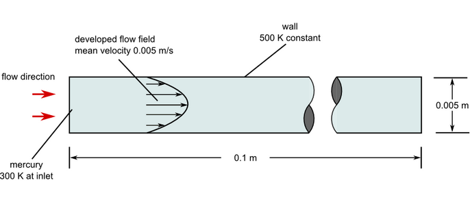
Figure 1. Critical Dimensions and Parameters for Simulating Laminar Flow through a Pipe with Constant Wall Temperature
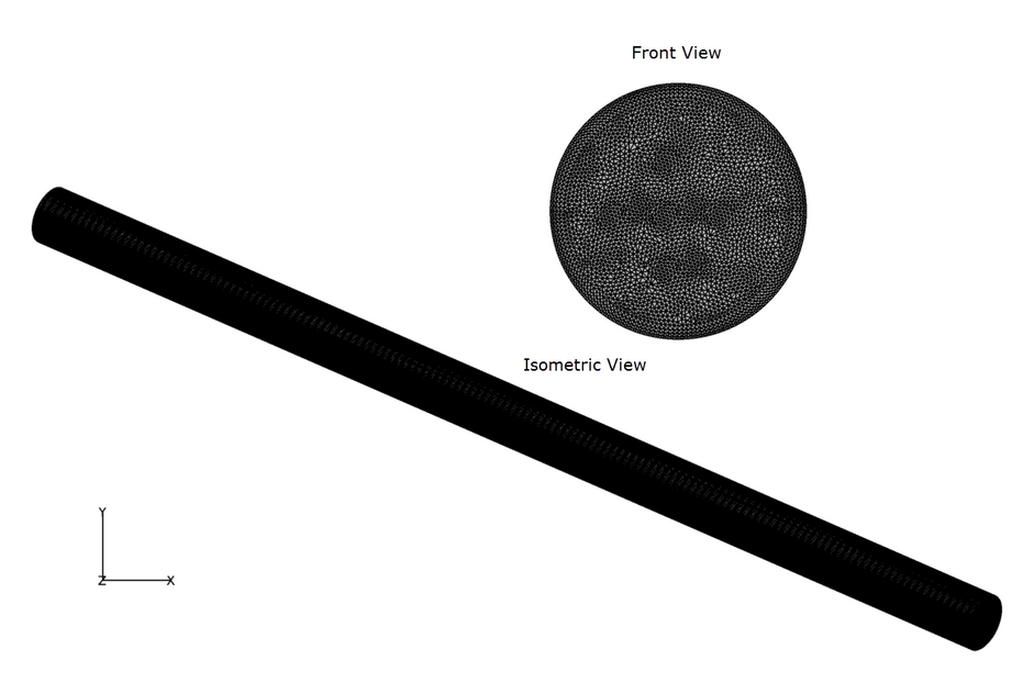
Figure 2. Mesh used for Simulating Laminar Flow Through a Pipe with Constant Wall Temperature
AcuSolve Results
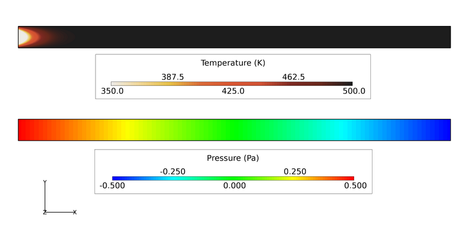
Figure 3. Temperature and Pressure Contours of Mercury Flow Through a Pipe with Prescribed Temperature Boundary
| Analytical solution | AcuSolve solution | Percent deviation from analytical | |
|---|---|---|---|
| Pressure drop (Pa) | 0.991 | 0.9925 | 0.15 |
| Centerline temperature of flow at outlet (K) | 500.0 | 500.0 | < 0.0001 |
Summary
The AcuSolve solution compares well with analytical results for flow through a pipe with constant temperature boundary conditions. The AcuSolve solution for the centerline temperature is nearly identical with the analytical results and the pressure reduces as expected for the prescribed flow conditions. The results of this simulation validate the ability of AcuSolve to accurately predict the heating of fluid flowing through a pipe with constant wall temperature.
Simulation Settings for Laminar Flow Through a Pipe With Constant Wall Temperature
AcuConsole database file: <your working directory>\pipe_laminar_heatDirichlet\pipe_laminar_heatDirichlet.acs
Global
- Problem Description
- Analysis type - Steady State
- Temperature equation - Advective Diffusive
- Turbulence equation - Laminar
- Auto Solution Strategy
- Relaxation Factor - 0.2
- Material Model
- Mercury
- Density - 13579.0 kg/m3
- Specific Heat - 139.3 J/kg-K
- Viscosity - 0.001548 kg/m-sec
- Conductivity - 8.69 W/m-K
Model
- Mercury
- Volume
- Fluid
- Element Set
- Material model - Mercury
- Element Set
- Fluid
- Surfaces
- Inflow
- Simple Boundary Condition - (disabled to allow for periodic conditions to be set)
- Advanced Options
- Integrated Boundary Conditions
- Mass Flux
- Type - Constant
- Constant value - 1.33e-3 kg/sec
- Mass Flux
- Temperature
- Type - Constant
- Constant value - 300.0 K
- Integrated Boundary Conditions
- Outflow
- Simple Boundary Condition - (disabled to allow for periodic conditions to be set)
- Wall
- Simple Boundary Condition
- Type - Wall
- Temperature BC type - Value
- Temperature - 500.0 K
- Simple Boundary Condition
- Inflow
- Periodics
- Periodic 1
- Individual Periodic BCs
- Velocity
- Type - Periodic
- Pressure
- Type - Single Unknown Offset
- Velocity
- Individual Periodic BCs
- Periodic 1
References
F. M. White. "Fluid Mechanics". 3rd Edition. McGraw-Hill Book Co., Inc. New York. 1994.
F. P. Incropera and D. P. DeWitt. "Fundamentals of Heat Transfer". John Wiley & Sons. New York. 1981.