ELEMENT_SET
Specifies a set of elements.
Type
AcuSolve Command
Syntax
ELEMENT_SET ("name") {parameters}
Qualifier
User-given name.
Parameters
- shape (enumerated) [no default]
- Topology of the elements in the set. Used only when the elements are specified
using the elements option.
- four_node_tet or tet4
- Four-node tetrahedron.
- five_node_pyramid or pyramid5
- Five-node pyramid.
- six_node_wedge or wedge6
- Six-node wedge (prism).
- eight_node_brick or hex8
- Eight-node brick (hexahedron).
- ten_node_tet or tet10
- Ten-node tetrahedron.
- elements (array) [no default]
- A set of element connectivity.
- volume_sets (list) [={}]
- List of volume set names (strings) to use in this element set. When using this option, the connectivity and shape of the elements are provided by the volume set container and it is unnecessary to specify the shape and elements options directly to the ELEMENT_SET command. In general, this option is used in place of directly specifying the shape and elements parameters in the ELEMENT_SET command. In the event that both the volume_sets and elements parameters are provided, the full collection of elements is read and a warning message is issued. The volume_sets option is the preferred method to specify the elements for the element set. This option provides support for mixed element topologies within a given element set and simplifies pre-processing and post-processing.
- medium (enumerated) [=fluid]
- Type of physics being solved.
- none
- No medium. Deactivates element set.
- fluid
- Fluid medium. Requires material_model.
- multi_field
- Multi-fluid medium. Requires multi_field_model.
- solid
- Solid medium. Solve only for temperature field. Requires material_model.
- shell
- Shell medium. Solve only for temperature field. Requires num_shell_layers, shell_material_models, shell_thickness_type and shell_thicknesses.
- quadrature (enumerated) [=full]
- Quadrature rule used to integrate the element contribution.
- reduced
- Reduced quadrature.
- full
- Full quadrature.
- high_1
- High-order quadrature.
- high_2
- High-order quadrature (higher than high_1).
- nodal
- Nodal quadrature.
- material_model or material (string) [no default]
- User-given name of the material model to be used in this element set. Used for fluid and solid media.
- multi_field_model (string) [no default]
- User-given name of the multi field model to be used in this element set. Used only for multi_field medial.
- body_force (string) (string)
- User-given name of the volumetric body force to be applied to this element set. If none, no body force is applied.
- element_volume_heat_sources (array) [={}]
- Heat source per unit volume given on a per-element basis in a two-column array. This option is not supported with mixed topology element sets.
- element_volume_momentum_sources (array) [={}]
- Momentum source per unit volume given on a per-element basis in a four-column array. This option is not supported with mixed topology element sets.
- reference_frame (string) [=none]
- User-given name of the reference frame for this element set. If none, the fixed reference frame is used.
- mesh_motion (string) [=none]
- User-given name of the MESH_MOTION command for specifying mesh displacement boundary conditions on all the nodes in this element set. If none, no boundary conditions are imposed.
- mesh_motion_precedence (integer) >=0 [=0]
- Precedence of the given mesh motion. When specifying the mesh motion on an element set level, all nodes within the set, including the boundary nodes, inherit the mesh motion. For applications where the surface nodes of the volume have a conflicting mesh motion constraint that is specified through the SIMPLE_BOUNDARY_CONDITION or NODAL_BOUNDARY_CONDITION command, the mesh_motion_precedence is used to resolve the conflict. The constraint with the highest precedence takes priority. The default value of mesh_motion_precedence is equal to zero, indicating that SIMPLE_BOUNDARY_CONDITION and NODAL_BOUNDARY_CONDITION constraints will take priority. Their default precedence is 1. In the case of equal precedence values, the SIMPLE_BOUNDARY_CONDITION and NODAL_BOUNDARY_CONDITION constraints will override those set on the ELEMENT_SET level.
- num_shell_layers or layers (integer)>0 [=1]
- Number of layers in the shell. Used for shell medium only.
- shell_material_models (list) [={}]
- List of material model names (strings) for the shell layers. Number of entries in the list must equal num_shell_layers. Used for shell medium only.
- shell_thickness_type (enumerated) [=constant]
- Type of shell thickness. Used for shell medium only.
- constant or const
- Constant shell thickness.
- shell_thicknesses or thick (array) [={}]
- Thicknesses of the shell layers. Number of entries in the array must equal num_shell_layers. Used with constant shell thickness type and for shell medium only.
- viscous_heating (boolean) [=off]
- Flag specifying whether to add the viscous heating term in the temperature equation.
- compression_heating (boolean) [=off]
- Flag specifying whether to add the compression heating term in the temperature equation.
- residual_control (boolean) [=on]
- Flag specifying whether to use nonlinear residual control to further stabilize the algorithm.
- oscillation_control (boolean) [=on]
- Flag specifying whether to use oscillation control to further stabilize the temperature, species, and turbulence equations.
- mesh_distortion_correction_factor (real) >=0 [=0]
- Amount of correction to be applied to the element Jacobian of highly distorted elements.
- mesh_distortion_tolerance (real) >=0 [=0]
- Determines if correction needs to be applied to the element Jacobian for highly distorted elements.
- auxiliary_elements (array) [no default]
- Element connectivity for auxiliary elements. Used with element user-defined functions. This option is not supported with mixed topology element sets.
- auxiliary_material_model (string) [no default]
- User-given name of the material model to be used for the auxiliary elements. This option is not supported with mixed topology element sets.
- auxiliary_reference_frame (string) [=none]
- User-given name of the reference frame to be used for the auxiliary elements. This option is not supported with mixed topology element sets.
- turbulence_suppression (boolean) [=off]
- Flag specifying whether to suppress turbulence production and ignore the contribution of eddy viscosity in a turbulence model.
Description
ELEMENT_SET( "air flow" ) {
   elements            = { 1001, 1, 2, 4, 3, 11, 12, 14, 13 ;
                           1002, 3, 4, 6, 5, 13, 14, 16, 15 ;
                           1003, 5, 6, 8, 7, 15, 16, 18, 17 ; }
   medium              = fluid
   shape               = eight_node_brick
   quadrature          = full
   material_model      = "air at standard temperature"
   reference_frame     = none
   mesh_motion         = none
   body_force          = none
   residual_control    = on
   oscillation_control = on
}
specifies an element set with three eight-node brick fluid elements.
VOLUME_SET( "tetrahedra" ) {
   elements  = { 1, 1, 2, 4, 3 ;
                 2, 3, 4, 6, 5 ;
                 3, 5, 6, 8, 7 ; }
   shape     = four_node_tet
}
VOLUME_SET( "prisms" ) {
   elements  = { 1, 1, 2, 4,  9, 10, 11 ;
                 2, 3, 4, 6, 12, 13, 14 ;
                 3, 5, 6, 8, 15, 16, 17 ; }
   shape     = six_node_wedge
}ELEMENT_SET( "fluid elements" ) {
volume_sets = {"tetrahedra","prisms"}
medium = fluid
quadrature = full
material_model = "air at standard temperature"
reference_frame = none
mesh_motion = none
body_force = none
residual_control = on
oscillation_control = on
}tetrahedra
prismsELEMENT_SET( "fluid elements" ) {
volume_sets = Read("volume_sets.vst")
medium = fluid
quadrature = full
material_model = "air at standard temperature"
reference_frame = none
mesh_motion = none
body_force = none
residual_control = on
oscillation_control = on
}The mixed topology version of the ELEMENT_SET command is preferred. This version provides support for multiple element topologies within a given element set and simplifies pre-processing and post-processing. In the event that both the volume_sets and elements parameters are provided in the same instance of ELEMENT_SET, the full collection of elements is read and a warning message is issued. Although the single and mixed topology formats of the commands can be combined, it is strongly recommended that they are not.
In the examples above, full quadrature rule is used. The "air at standard temperature" material model is applied. The elements are in the fixed reference frame and not subject to mesh motion. No body force is added. Both the residual and oscillation controls are turned on.
The medium parameter specifies whether the element set is of type fluid, solid, shell, or none. A fluid element set solves for all equations in the system. A solid or shell element set solves only the temperature and mesh displacement equations, while all other equations, such as flow, turbulence, and species, are ignored. Therefore, appropriate boundary conditions at the interface of the fluid and solid/shell elements must be imposed. A type of none effectively deactivates the element set and all of its associated surfaces; the elements do not contribute to any equation. The nodes may still be moved through the use of the mesh_motion parameter. The element set may be reactivated by changing its type on restart.
For all forms of the command, the material_model parameter is mandatory. When defining the elements using the single topology form of the command, the elements and shape parameters are also mandatory. shape specifies the shape (topology) of the elements in the set. elements provide the element connectivity. This parameter is a multi column array, with one row per element. The first column corresponds to the element numbers, which are unique numbers within this element set. Negative values are acceptable. The remaining columns are the element nodes. The number of element nodes and their order must match the shape of the element set. The element node numbers must be valid numbers, as given by the COORDINATE command.
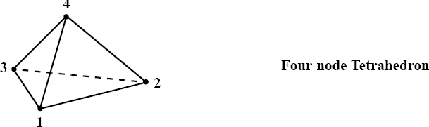
Figure 1. Four-node Tetrahedron Element
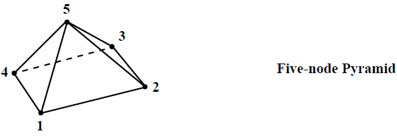
Figure 2. Five-node Pyramid Element
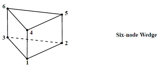
Figure 3. Six-node Wedge Element
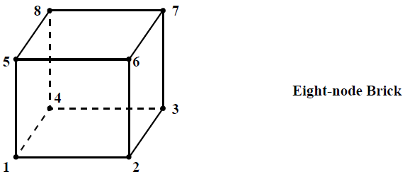
Figure 4. Eight-node Brick Element
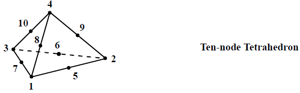
Figure 5. Ten-node Tetrahedron Element
1001      1   2    4   3   11   12    14     13
1002      3   4    6   5   13   14    16     15
1003 5 6 8 7 15 16 18 17ELEMENT_SET( "air flow" ) {
elements = Read( "air.cnn" )
medium = fluid
shape = eight_node_brick
material_model = "air at standard temperature"
}| Shape | Quadrature rule | ||||
|---|---|---|---|---|---|
| full | reduced | nodal | high_1 | high_2 | |
| four_node_tet | 4-point | 1-point | 4-point nodal | 14-point | 20-point |
| five_node_pyramid | 5-point | 1-point | 5- point nodal | 13-point | 13-point |
| six_node_wedge | 3x2 | 2-point | 6-point nodal | 6x3 | 7x4 |
| eight_node_brick | 2x2x2 | 2x2x 2 | 8-point nodal | 3x3x3 | 4x4x 4 |
| ten_node_tet | 8-point | 4-point | 10-point nodal | 20-point | 35-point |
ELEMENT_SET( "HIGH QUAD 1" )
   ...
   quadrature      = high_1
   ...
}ELEMENT_SET( "air flow" ) {
material_model = "air at standard temperature"
...
}
MATERIAL_MODEL( "air at standard temperature" ) {
...
}By default, all element sets are defined with respect to the fixed, or "laboratory", reference frame. If the REFERENCE_FRAME command is used to define the rotational body forces, this is recommended, as opposed to using the ROTATION_FORCE command, then reference_frame is used to define the reference frame for the element set. In this case the body_force command referenced by the body_force parameter (see below) should not include the rotation_force parameter, since rotational forces have already been included. See the REFERENCE_FRAME command for more details and an example.
ELEMENT_SET( "rotating fan" ) {
   mesh_motion       = "rotating fan"
   ...
}
MESH_MOTION( "rotating fan" ) {
   type              = rotation
   rotation_center   = { 0, 0, 0 }
   angular_velocity  = { 0, 3, 0 }
}
Note the important difference between reference_frame and mesh_motion: the former introduces an accelerating reference frame and modifies the velocity field while the latter moves the mesh through the reference frame. For complex problems both may be used simultaneously, although great care needs to be exercised.
ELEMENT_SET( "air flow" ) {
   body_force        = "added heat"
   ...
}
BODY_FORCE( "added heat" ) {
   mass_heat_source  = "my heat source"
}ELEMENT_SET( "air flow" ) {
...
element_volume_heat_sources = { 1, 1.5 ;
2, 2.5 ;
3, 3.5 }
}where the first column contains the element numbers and the second column contains the volume heat source data.
A shell medium is used to model the energy equation in solid materials where the thinness of the geometry makes it inconvenient to use a solid medium. The shell medium supports only wedges and bricks. The triangular faces of the wedges must be on the outside surfaces of the shell. Geometrically, the shell is infinitely thin, so that the pairs of nodes in an element that are on opposite sides of the shell have the same coordinates. These nodes normally need to have different node numbers in order to support temperature and pressure differences across the shell, but in cases where no such differences exist (for example, an edge of a shell that is surrounded by fluid) they would share the same node number. Such "collapsed" elements are not supported for fluid and solid media. The first three (for wedges) or four (for bricks) nodes of the connectivity define the first face of the shell and the last three or four nodes define the second face. Between these faces, the element is divided up into a number of layers, given by num_shell_layers. The first layer of the shell is adjacent to the first face, the last (num_shell_layers) is next to the second face and the others are placed in order in between. Each layer is assigned a material model and a thickness through the shell_material_models and shell_thicknesses parameters. Both of these must be specified and both are arrays where the layer data must be given in order. material_model is ignored for shells.
Two important assumptions are made for shells. First, the thicknesses parameter always applies in the direction perpendicular to the surface of the shell on an element basis. This might be inaccurate for thick shells and tightly curved surfaces. Second, the intermediate temperatures needed at the quadrature points of each layer are calculated based on a simplified analysis. A one-dimensional heat equation through the shell thickness at the element nodes is derived by neglecting thermal inertia and conduction parallel to the surface. This means that the heat flux is the same in all the layers. If each layer material model has a constant conductivity, then this simplified heat equation is solved exactly. If any of the conductivities is a function of temperature, then a two-pass procedure is used to approximately solve the resulting nonlinear system. Once the temperatures are known at the corners of all the layers in each element, then they can be interpolated to the quadrature points in the usual manner. Note that the assumptions used to obtain the intermediate temperatures do not apply to the overall formulation for the shells. That is, thermal inertia, multi-dimensional conduction, and nonlinearities are all modeled accurately in the final solution.
MATERIAL_MODEL( "layer 1" ) {
   density_model          = "layer 1"
   specific_heat_model    = "layer 1"
   conductivity_model     = "layer 1"
}
MATERIAL_MODEL( "layer 2" ) {
   density_model          = "layer 2"
   specific_heat_model    = "layer 2"
   conductivity_model     = "layer 2"
}
ELEMENT_SET( "shells" ) {
   elements               = Read( "shell.shl.cnn" )
   shape                  = eight_node_brick
   quadrature             = full
   medium                 = shell
   num_shell_layers       = 2
   shell_thicknesses      = { 5.e-3, 2.e-3 }
   shell_material_models  = { "layer 1", "layer 2" }
}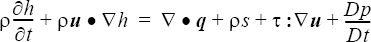
See the EQUATION command for a description of the individual terms. The last term is the material derivative of pressure and known as the compression heating term, and the adjacent term is the viscous heating term. These are both turned off by default and are important in only limited cases such as extremely viscous flows and variable density material models. Care should be exercised in activating these terms in conjunction with turbulent flows. They are evaluated as written (using the turbulent viscous stress tensor for τ), although optimally each of these terms should be modeled as a whole.
The residual_control and oscillation_control parameters add stabilization terms to the finite element formulation. The residual control option adds the so-called "discontinuity capturing" operator to all fluid equations. This operator controls unresolved internal and boundary discontinuities. The oscillation control option adds a nonlinear maximum principal operator onto the advective term of the scalar (temperature, species, and turbulence) equations, which helps to control any spurious oscillations. These two operators are turned on by the defaults and they should be rarely turned off.
ELEMENT_SET( "PINCHED TUBE" ) {
   ...
   mesh_distortion_correction_factor = 1.0e-4
   mesh_distortion_tolerance         = 1.0e-2
   ...
}
Considering the settings shown above, AcuSolve allows element Jacobians to decrease to a level of -1.0e-4 before terminating the simulation (when mesh=specified, or mesh=eulerian) or adding non-linear iterations to the mesh displacement stagger (when mesh=ale).
When the element Jacobian satisfies the following relationship:
0 >= element Jacobian > -mesh_distortion_tolerance, and the mesh_distortion_correction_factor is non-zero, the element Jacobian is adjusted. Using this approach, a target Jacobian is computed that is proportional to mesh_distortion_correction_factor. The actual element Jacobian is then perturbed to match the target Jacobian. The larger the mesh_distortion_correction_factor, the further the Jacobain deviates from the true value. This has two implications. The first is that the flow solver will continue running with more highly distorted elements (a higher degree of penetrating faces). The second is that the solution in the impacted elements may deviate further from what it should be considering the actual location of the nodes. Therefore, this option should be used cautiously. It should also be noted that this approach does not actually adjust the position of the nodes. Rather, it enforces a correction on the Jacobian of the element that allows the flow solver to continue without exiting when a negative Jacobian is encountered.
Several commands, such as ELEMENT_BOUNDARY_CONDITION and SURFACE_OUTPUT, require element surfaces. These surfaces are defined with respect to the elements of an ELEMENT_SET command. In addition to their geometrical connection, these commands also inherit the quadrature rule, material models, and other attributes of the element set.
ELEMENT_SET( "radiator element set" ) {
   ...
}
HEAT_EXCHANGER_COMPONENT( "radiator" ) {
   element_set    = "radiator element set"
   ...
}
turns the element set "radiator element set" into a radiator. In such cases, the element set must contain all the elements of the component and no other elements. Moreover, the element set may be referenced by only one component command.
ELEMENT_SET( "air" ) {
   elements                   = { 1, 1, 2, 3, 4 ;
                                  2, ... ;
                                  3, ... ; }
   shape                      = four_node_tet
   medium                     = fluid
   material_model             = "air"
   body_force                 = "air/fin heat transfer"
   auxiliary_elements         = { 1, 11, 12, 13, 14 ;
                                  2, ... ; 3, ... ; }
   auxiliary_material_model   = "fin"
   auxiliary_reference_frame  = none
}
ELEMENT_SET( "fin" ) {
   elements                   = { 1001, 11, 12, 13, 14 ;
                                  1002, ... ;
                                  1003, ... ; }
   shape                      = four_node_tet
   medium                     = fluid
   material_model             = "fin"
   body_force                 = "fin/air heat transfer"
   auxiliary_elements         = { 1001, 1, 2, 3, 4 ; 1002, ... ; 1003, ... ; }
   auxiliary_material_model   = "air"
   auxiliary_reference_frame  = none
}
BODY_FORCE( "air/fin heat transfer" ) {
   mass_heat_source          = "air/fin heat transfer"
}
MASS_HEAT_SOURCE( "air/fin heat transfer" ) {
   type                       = user_function
   user_function              = "usrFinAirHeat"
   user_values                = { 1 , # 1: air side, 2: fin side
                                  1.e6/1.225 } # coefficient
}
BODY_FORCE( "fin/air heat transfer" ) {
   mass_heat_source           = "fin/air heat transfer"
}
MASS_HEAT_SOURCE( "fin/air heat transfer" ) {
   type                       = user_function
   user_function              = "usrFinAirHeat"
   user_values                = { 2 , # 1: air side, 2: fin side
                                  1.e6/8666 } # coefficient
}1 11
2 12
3 13
4 141 11 12 13 14
2 ...
3 ...ELEMENT_SET( "air" ) {
...
auxiliary_elements = Read( "aux_fin.cnn" )
auxiliary_material_model = "fin"
auxiliary_reference_frame = none
}#include "acusim.h"
#include "udf.h"
UDF_PROTOTYPE( usrFinAirHeat ) ; /* function prototype */
Void usrFinAirHeat (
UdfHd udfHd, /* Opaque handle for accessing data */
Real* outVec, /* Output vector */
Integer nItems, /* Number of elements in this block */
Integer vecDim /* = 1 */
) {
Integer elem ; /* an element counter */
Integer side ; /* which side of heat transfer? */
Real fct ; /* scaling factor */
Real hCoef ; /* modified heat transfer coefficient */
Real heatCoef ; /* heat transfer coefficient */
Real* airTemp ; /* air temperature */
Real* airVel ; /* air velocity */
Real* crd ; /* coordinates */
Real* finTemp ; /* fin temperature */
Real* srcJac ; /* partial heat source / partial temp */
Real* usrVals ; /* user values */
/* Get the data */ */
udfCheckNumUsrVals( udfHd, 2 ) ; /* check for error */
usrVals = udfGetUsrVals( udfHd ) ; /* get the user vals */
side = (Integer) usrVals[0] ; /* get the side */
heatCoef = usrVals[1] ; /* get the heat coef. */
/* Get the material data */
if ( side == 1 ) { /* air side */
airTemp = udfGetElmData( udfHd, UDF_ELM_TEMPERATURE ) ;
airVel = udfGetElmData( udfHd, UDF_ELM_VELOCITY ) ;
finTemp = udfGetElmAuxData( udfHd UDF_ELM_TEMPERATURE ) ;
srcJac = udfGetElmJac( udfHd, UDF_ELM_JAC_TEMPERATURE ) ;
crd = udfGetElmCrd( udfHd ) ;
fct = 1. ;
} else {
airTemp = udfGetElmAuxData( udfHd, UDF_ELM_TEMPERATURE ) ;
airVel = udfGetElmAuxData( udfHd, UDF_ELM_VELOCITY ) ;
finTemp = udfGetElmData( udfHd, UDF_ELM_TEMPERATURE ) ;
srcJac = udfGetElmJac( udfHd, UDF_ELM_JAC_TEMPERATURE ) ;
crd = udfGetElmAuxCrd( udfHd ) ;
fct = -1. ;
}
/* Compute the heat flux */
for ( elem = 0 ; elem < nItems ; elem++ ) {
hCoef = heatCoef ; /* could be a function of airVel */
outVec[elem] = fct * hCoef * ( finTemp[elem] - airTemp[elem]);
srcJac[elem] = -hCoef ;
}
} /* end of usrFinAirHeat() */The dimension of the returned coefficient vector, outVec, is the number of elements.