HEAT_EXCHANGER_COMPONENT
Specifies a heat exchanger component for an element set.
Type
AcuSolve Command
Syntax
HEAT_EXCHANGER_COMPONENT("name") {parameters...}
Qualifier
User-given name.
Parameters
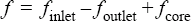
- type (enumerated) [=constant_coolant_heat_reject]
- Type of heat exchanger model to use.
- constant_coolant_heat_reject
- Constant heat rejection. Requires coolant_heat_reject.
- constant_coolant_temperature
- Constant coolant temperature. Requires coolant_temperature.
- shape (enumerated) [no default]
- Shape of the surfaces.
- three_node_triangle or tri3
- Three-node triangle.
- four_node_quad or quad4
- Four-node quadrilateral
- six_node_triangle or tri6
- Six-node triangle.
- element_set or elem_set (string) [no default]
- User-given name of the parent element set. This element set is turned into a heat exchanger component by this command.
- surfaces (array) [no default]
- List of component inlet element surfaces.
- surface_sets (list) [={}]
- List of surface set names (strings) to use in this heat exchanger component. When using this option, the connectivity, shape, and parent element of the surfaces are provided by the surface set container and it is unnecessary to specify the shape, element_set and surfaces parameters directly to the HEAT_EXCHANGER_COMPONENT command. This option is used in place of directly specifying these parameters. In the event that both the surface_sets and surfaces parameters are provided, the full collection of surface elements is read and a warning message is issued. The surface_sets option is the preferred method to specify the surface elements. This option provides support for mixed element topologies and simplifies pre-processing and post-processing.
- coolant_heat_reject or heat_reject (real) [=0]
- The amount of heat rejected by the heat exchanger. Used with constant_coolant_heat_reject type.
- coolant_temperature (real) [=0]
- The temperature of the heat exchanger coolant. Used with constant_coolant_temperature type.
- coolant_heat_reject_multiplier_function (string) [=none]
- User-given name of the multiplier function for scaling the amount of heat rejected by the heat exchanger. If none, no scaling is performed.
- coolant_temperature_multiplier_function (string) [=none]
- User-given name of the multiplier function for scaling the coolant temperature. If none, no scaling is performed.
- coolant_flow_rate or flow_rate (real) >=0 [=0]
- Flow rate of the coolant liquid.
- coolant_flow_rate_multiplier_function (string) [=none]
- User-given name of the multiplier function for scaling the flow rate of the coolant liquid. If none, no scaling is performed.
- direction or dir (array) [={1,0,0}]
- Direction of the flow through the heat exchanger.
- thickness (real) >0 [=1]
- Thickness of the heat exchanger: the distance from the inlet surface to the outlet surface.
- upstream_distance (real) >=0 [=0]
- Distance in front of the heat exchanger inlet surface at which the upstream temperature is sampled.
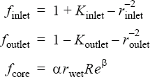
- friction_type (enumerated) [=constant]
- Type of the friction factor model.
- constant or const
- Constant friction factor. Requires friction.
- kays_london
- Kays-London friction factor. Requires wet_min_area_ratio, core_friction_constant, core_friction_exponent, inlet_loss_coefficients and outlet_loss_coefficients.
- piecewise_linear or linear
- Piecewise linear curve fit. Requires friction_curve_fit_values and friction_curve_fit_variable.
- cubic_spline or spline
- Cubic spline curve fit. Requires friction_curve_fit_values and friction_curve_fit_variable.
- user_function or user
- User-defined function. Requires friction_user_function, friction_user_values, and friction_user_strings.
- friction (real) [=0]
- Constant value of the friction factor. Used with constant friction type.
- inlet_min_area_ratio (real) >0 [=1]
- Ratio of inlet area to minimum flow area.
- outlet_min_area_ratio (real) >0 [=1]
- Ratio of outlet area to minimum flow area. This typically is equal to inlet_min_area_ratio
- wet_min_area_ratio (real) >0 [=1]
- Ratio of the wetted area to minimum flow area. Used with kays_london friction type.
- core_friction_constant (real) >=0 [=1]
- Constant coefficient of the core friction factor. Used with kays_london friction type.
- inlet_loss_coefficients (array) [={0.4,0.0,-0.4}]
- Loss coefficients for the inlet friction factor. This is a 3-component array corresponding to the constant, linear, and quadratic coefficients. Used with kays_london friction type.
- outlet_loss_coefficients (array) [={1,-2,1}]
- Loss coefficients for the outlet friction factor. This is a three component array corresponding to the constant, linear and quadratic coefficients. Used with kays_london friction type.
- core_friction_exponent (real) [=-1]
- Exponential coefficient of the core friction factor. Used with kays_london friction type.
- friction_curve_fit_values (array) [={0,1}]
- A two column array of independent-variable/friction-factor data values. Used with piecewise_linear and cubic_spline friction types.
- friction_curve_fit_variable (enumerated) [=axial_velocity]
- Independent variable of the friction factor curve fit. Used with
piecewise_linear and cubic_spline
friction types.
- axial_velocity
- Velocity in the direction of the component.
- friction_user_function (string) [no default]
- Name of the friction factor user-defined function. Used with user_function friction type.
- friction_user_values (array) [={}]
- Array of values to be passed to the friction factor user-defined function. Used with user_function friction type.
- friction_user_strings (list) [={}]
- Array of strings to be passed to the friction factor user-defined function. Used with user_function friction type.
- friction_multiplier_function (string) [=none]
- User-given name of the multiplier function for scaling the friction factor. If none, no scaling is performed.
- transverse_friction_factor (real) >=0 [=10]
- Fraction of the friction factor used for the transverse friction factor. Higher values yield higher degrees of unidirectional flow, but comes at the expense of stability.
- effectiveness_type (enumerated) [=constant]
- Type of the thermal effectiveness.
- constant or const
- Constant for the entire set. Requires effectiveness.
- piecewise_bilinear or bilinear
- Piecewise bilinear curve fit. Requires effectiveness_curve_fit_values, effectiveness_curve_fit_row_variable and effectiveness_curve_fit_column_variable.
- user_function or user
- User-defined function. Requires effectiveness_user_function and effectiveness_user_strings.
- effectiveness (real) [=1]
- The constant value of the thermal effectiveness. Used with constant effectiveness.
- effectiveness_curve_fit_values (array) [={0,0;0,1}]
- Effectiveness as a two dimensional curve fit table with two independent variables. Used with piecewise_bilinear effectiveness type.
- effectiveness_curve_fit_row_variable (enumerated) [=coolant_flow_rate]
- Independent variable of the rows of the effectiveness curve fit table. Used
with piecewise_bilinear effectiveness type.
- coolant_flow_rate
- Coolant flow rate.
- effectiveness_curve_fit_column_variable (enumerated) [=axial_velocity]
- Independent variable of the columns of the effectiveness curve fit table.
Used with piecewise_bilinear effectiveness type.
- axial_velocity
- Velocity in the direction of the component.
- effectiveness_user_function (string) [no default]
- Name of the user-defined function for the thermal effectiveness. Used with user_function effectiveness type.
- effectiveness_user_values (array)[={}]
- Array of values to be passed to the thermal effectiveness user-defined function. Used with user_function effectiveness type.
- effectiveness_user_strings (list) [={}]
- Array of strings to be passed to the thermal effectiveness user-defined function. Used with user_function effectiveness type.
- effectiveness_multiplier_function (string) [=none]
- User-given name of the multiplier function for scaling the thermal effectiveness. If none, no scaling is performed.
Description
ELEMENT_SET( "radiator" ) {
    shape = four_node_tet
    elements = { 1, 1, 9, 8, 3 ;
                 2, 3, 8, 9, 5 ;
                 ... }
    ...
}
HEAT_EXCHANGER_COMPONENT( "radiator component" ) {
    shape                            = three_node_triangle
    element_set                      = "radiator"
    surfaces                         = { 1, 101, 1, 9, 8 ;
                                         2, 102, 8, 9, 5 ; }
    type                             = constant_coolant_heat_reject
    coolant_heat_reject              = 237443.5
    coolant_flow_rate                = 4.6
    direction                        = { 1, 0, 0 }
    thickness                        = 0.1
    upstream_distance                = 0.05
    friction_type                    = kays_london
    inlet_min_area_ratio             = 1.296
    outlet_min_area_ratio            = 1.296
    wet_min_area_ratio               = 54.18
    core_friction_constant           = 23.505
    core_friction_exponent           = -.74
    inlet_loss_coefficients          = { 0.4, 0.0, -0.4 }
    outlet_loss_coefficients         = { 1.0, -2., 1.0 }
    transverse_friction_factor       = 100
    effectiveness_type               = piecewise_bilinear
    effectiveness_curve_fit_values   = {
              0 ,  1.0000, 3.0000, 5.0000, 7.5000, 10.000, 13.500 ;
              0.4, 0.7487, 0.3302, 0.2511, 0.1731, 0.1411, 0.0987 ;
              1.1, 0.8877, 0.5422, 0.4301, 0.3021, 0.2524, 0.1822 ;
              1.7, 0.9123, 0.6321, 0.5332, 0.3923, 0.3387, 0.2487 ;
              2.6, 0.9344, 0.6953, 0.5962, 0.4693, 0.4023, 0.3084 ;
              3.5, 0.9452, 0.7233, 0.6287, 0.4976, 0.4344, 0.3329 ;
    effectiveness_curve_fit_row_variable = coolant_flow_rate
    effectiveness_curve_fit_column_variable = axial_velocity
}
turns the "radiator" element set into a heat exchanger component. The inlet to this heat exchanger is defined by the two surfaces (element faces) of elements one and two. The heat exchanger flows in the positive global x-direction. The heat exchanger transfers 237443.5 units of energy from the coolant to the flow. The coolant flow rate is 4.6. The component thickness is 0.1. The upstream temperature is sampled 0.05 coordinate units in front of the component inlet surface. The Kays-London model is used to incorporate the heat exchanger friction. A two dimensional curve fit is used to model the heat transfer effectiveness from the coolant to the flow.
- Element Shape
- Surface Shape
- four_node_tet
- three_node_triangle
- five_node_pyramid
- three_node_triangle
- five_node_pyramid
- four_node_quad
- six_node_wedge
- three_node_triangle
- six_node_wedge
- four_node_quad
- eight_node_brick
- four_node_quad
- ten_node_tet
- six_node_triangle
The surfaces parameter contains the faces of the element set. This parameter is a multi-column array. The number of columns depends on the shape of the surface. For three_node_triangle, this parameter has five columns, corresponding to the element number (of the parent element set), a unique (within this set) surface number, and the three nodes of the element face. For four_node_quad, surfaces has six columns, corresponding to the element number, a surface number, and the four nodes of the element face. For six_node_triangle, surfaces has eight columns, corresponding to the element number, a surface number, and the six nodes of the element face. One row per surface must be given. The three, four, or six nodes of the surface may be in any arbitrary order, since they are reordered internally based on the parent element definition.
1 101 1 9 8
2 102 8 9 5HEAT_EXCHANGER_COMPONENT( "radiator component" ) {
shape = three_node_triangle
element_set = "radiator"
surfaces = Read( "radiator.srf" )
...
}SURFACE_SET( "tri faces" ) {
surfaces = { 1, 1, 1, 2, 4 ;
2, 2, 3, 4, 6 ;
3, 3, 5, 6, 8 ; }
shape = three_node_triangle
volume_set = "tetrahedra"
}
SURFACE_SET( "quad faces" ) {
surfaces = { 1, 1, 1, 2, 4, 9 ;
2, 2, 3, 4, 6, 12 ;
3, 3, 5, 6, 8, 15 ; }
shape = four_node_quad
volume_set = "prisms"HEAT_EXCHANGER_COMPONENT( "radiator component" ) {
surface_sets = {"tri_faces", "quad_faces"}
...
}tri faces
quad facesHEAT_EXCHANGER_COMPONENT( "radiator component" ) {
surface_sets = Read("surface_sets.srfst")
...
}The mixed topology version of the HEAT_EXCHANGER_COMPONENT command is preferred. This version provides support for multiple element topologies within a single instance of the command and simplifies pre-processing and post-processing. In the event that both the surface_sets and surfaces parameters are provided in the same instance of the command, the full collection of surface elements is read and a warning message is issued. Although the single and mixed topology formats of the commands can be combined, it is strongly recommended that they are not.
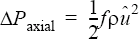
where  is the pressure drop in the heat exchanger axial
direction; the heat exchanger axial direction is specified by direction;
f is the friction factor, given by
friction_type and related parameters (see below);
ρ is the density;
u=rinletuaxial is
the axial velocity at the minimum cross-section area;
rinlet is the ratio of the
inlet area to the minimum cross-section area, given by
inlet_min_area_ratio; and
uaxial is the axial component
of the velocity.
is the pressure drop in the heat exchanger axial
direction; the heat exchanger axial direction is specified by direction;
f is the friction factor, given by
friction_type and related parameters (see below);
ρ is the density;
u=rinletuaxial is
the axial velocity at the minimum cross-section area;
rinlet is the ratio of the
inlet area to the minimum cross-section area, given by
inlet_min_area_ratio; and
uaxial is the axial component
of the velocity.
To confine the flow to remain in the direction of the heat exchanger, pressure drops in the transverse directions of the heat exchanger component are introduced. The friction factor of these directions is scaled by transverse_friction_factor.
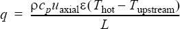

is equal to the heat exchanger heat rejection, specified by coolant_heat_reject. Here Ω is the heat exchanger volume.
A constant_coolant_heat_reject heat exchanger component adds a constant heat of coolant_heat_reject to the flow passing through the heat exchanger. The coolant flow is not modeled here; only its effect on the fluid flow is modeled.
HEAT_EXCHANGER_COMPONENT( "constant coolant temp radiator" ) {
    type                = constant_coolant_temperature
    coolant_temperature = 350.0
    ...
 }
The heat exchanger flow direction is given by direction, which is expressed in the global xyz coordinate system. The direction must be inward, normal to the heat exchanger inlet surface. This parameter is internally normalized.
thickness specifies the thickness (from the inlet to the outlet) of the heat exchanger. This thickness is assumed to be constant throughout the heat exchanger.
HEAT_EXCHANGER_COMPONENT( "constant friction radiator" ) {
  friction_type = constant
  friction      = 0.4
  ...
}
applies a constant friction factor of 0.4 to all the heat exchanger component elements.
Here Kinlet and Koutlet are the inlet and outlet loss coefficients, given by
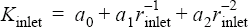
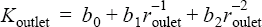
The coefficients 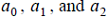 are specified by
inlet_loss_coefficients; the coefficients
are specified by
inlet_loss_coefficients; the coefficients 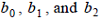 are specified by
outlet_loss_coefficients;
rinlet is the ratio of the
inlet area to the minimum cross section area, specified by
inlet_min_area_ratio; and
routlet is the ratio of the
outlet area to the minimum cross-section area, specified by
outlet_min_area_ratio.
are specified by
outlet_loss_coefficients;
rinlet is the ratio of the
inlet area to the minimum cross section area, specified by
inlet_min_area_ratio; and
routlet is the ratio of the
outlet area to the minimum cross-section area, specified by
outlet_min_area_ratio.


L is the heat exchanger thickness, specified by thickness.
HEAT_EXCHANGER_COMPONENT( "curve fit friction radiator" ) {
 friction_type             = piecewise_linear
 friction_curve_fit_values = { 0, 10.685 ;
                               5, 3.291 ;
                              10, 1.996 ;
                              15, 1.495 ;
                              20, 1.220 ;
                              30, 0.920 ;
                              40, 0.756 ;
                              50, 0.650 ; }
 friction_curve_fit_variable = axial_velocity
 ...
 }
defines the friction factor as a function of the axial velocity (that is, velocity in the direction of the heat exchanger). This curve fit is equivalent to the above Kays-London model, provided that the density is 1.225 and the dynamic viscosity is 1.781e-5. The friction_curve_fit_values parameter is a two-column array corresponding to the independent variable and the friction factor. The independent variable values must be in ascending order. The limit point values of the curve fit are used when friction_curve_fit_variable falls outside of the curve fit limits.
0 10.685
5 3.291
10 1.996
15 1.495
20 1.220
30 0.920
40 0.756
50 0.650HEAT_EXCHANGER_COMPONENT( "curve fit friction radiator" ) {
friction_type = piecewise_linear
friction_curve_fit_values = Read( "friction.fit" )
friction_curve_fit_variable = axial_velocity
...
}A friction factor of type user_function may be used to model more complex behaviors; see the AcuSolve User-Defined Functions Manual for a detailed description of user-defined functions.
HEAT_EXCHANGER_COMPONENT( "UDF friction radiator" ) {
 friction_type           = user_function
 friction_user_function  = "usrFrictionExample"
 friction_user_values    = { 1,0,0, # flow direction
                             0.0629, # constant
                            10.6225, # proportional
                            -0.74 } # exponential
 ...
}#include "acusim.h"
#include "udf.h"
UDF_PROTOTYPE( usrFrictionExample ) ; /* function prototype */
Void usrFrictionExample (
UdfHd udfHd, /* Opaque handle for accessing data */
Real* outVec, /* Output vector */
Integer nItems, /* Number of elements */
Integer vecDim /* = 1 */
) {
Integer elem ; /* an element counter */
Real aVel ; /* axial velocity */
Real coef1 ; /* constant coefficient */
Real coef2 ; /* proportional coefficient */
Real coef3 ; /* exponential coefficient */
Real xDir ; /* x-component of direction vector */
Real yDir ; /* y-component of direction vector */
Real zDir ; /* z-component of direction vector */
Real* spec ; /* specie field */
Real* usrVals ; /* user values */
Real* vel ; /* velocity field */
Real* xVel ; /* x-velocity */
Real* yVel ; /* y-velocity */
Real* zVel ; /* z-velocity */
udfCheckNumUsrVals( udfHd, 6 ) ; /* check for error */
usrVals = udfGetUsrVals( udfHd ) ; /* get the user vals */
xDir = usrVals[0] ; /* x-direction */
yDir = usrVals[1] ; /* y-direction */
zDir = usrVals[2] ; /* z-direction */
coef1 = usrVals[3] ; /* const. coeff. */
coef2 = usrVals[4] ; /* prop. coeff. */
coef3 = usrVals[5] ; /* exp. coeff. */
vel = udfGetElmData( udfHd, UDF_ELM_VELOCITY ) ; /* get velocity */
xVel = &vel[0*nItems] ; /* localized x-vel */
yVel = &vel[1*nItems] ; /* localized y-vel */
zVel = &vel[2*nItems] ; /* localized z-vel */
for ( elem = 0 ; elem < nItems ; elem++ ) {
aVel = xVel[elem] * xDir
+ yVel[elem] * yDir
+ zVel[elem] * zDir ;
outVec[elem] = coef1 + coef2 * pow( aVel, coef3 ) ;
}
} /* end of usrFrictionExample() */The dimension of the returned friction vector, outVec, is the number of elements.
The friction factor in the transverse direction is controlled by transverse_friction_factor. Ideally, an infinite friction factor should be imposed in the transverse direction, resulting in a unidirectional flow through the heat exchanger. This proves, however, to be unstable. Therefore a multiple of the friction factor in the axial direction is imposed instead. The multiplier is specified by transverse_friction_factor; values from 10 to 100 are typically used.
The amount of heat transferred from the coolant to the flow depends on the effectiveness of the heat exchanger, as given in the above equations.
HEAT_EXCHANGER_COMPONENT( "constant effectiveness radiator" ) {
  effectiveness_type = constant
  effectiveness      = 0.35
  ...
}0.7487 ... 0.0987
...
0.9452 ... 0.3329are the effectiveness coefficients.
0   1.0000 3.0000 5.0000 7.5000 10.000  13.500
0.4 0.7487 0.3302 0.2511 0.1731  0.1411  0.0987
1.1 0.8877 0.5422 0.4301 0.3021  0.2524  0.1822
1.7 0.9123 0.6321 0.5332 0.3923  0.3387  0.2487
2.6 0.9344 0.6953 0.5962 0.4693  0.4023  0.3084
3.5 0.9452 0.7233 0.6287 0.4976 0.4344 0.3329HEAT_EXCHANGER_COMPONENT( "radiator component" ) {
effectiveness_curve_fit_values = Read( "effectiveness.fit" )
...
}An effectiveness of type user_function allows for more complex behavior; see the AcuSolve User-Defined Functions Manual for a detailed description of user-defined functions.
HEAT_EXCHANGER_COMPONENT( "UDF effectiveness radiator" ) {
    effectiveness_type           = user_function
    effectiveness_user_function  = "usrEffectivenessExample"
    effectiveness_user_values    = { 1,0,0, # flow direction
                                         0.6, # coefficient 1
                                         0.9, # coefficient 2
                                         1.0 } # coefficient 3
    ...
}#include "acusim.h"
#include "udf.h"
UDF_PROTOTYPE( usrEffectivenessExample ) ; /* function prototype */
Void usrEffectivenessExample (
UdfHd udfHd, /* Opaque handle for accessing data */
Real* outVec, /* Output vector */
Integer nItems, /* Number of elements */
Integer vecDim /* = 1 */
) {
Integer elem ; /* an element counter */
Real aVel ; /* axial velocity */
Real coef1 ; /* rational function coefficient 1 */
Real coef2 ; /* rational function coefficient 2 */
Real coef3 ; /* rational function coefficient 3 */
Real xDir ; /* x-component of direction vector */
Real yDir ; /* y-component of direction vector */
Real zDir ; /* z-component of direction vector */
Real* usrVals ; /* user values */
Real* vel ; /* velocity field */
Real* xVel ; /* x-velocity */
Real* yVel ; /* y-velocity */
udfCheckNumUsrVals( udfHd, 6 ) ; /* check for error */
usrVals = udfGetUsrVals( udfHd ) ; /* get the user vals */
xDir = usrVals[0] ; /* x-direction */
yDir = usrVals[1] ; /* y-direction */
zDir = usrVals[2] ; /* z-direction */
coef1 = usrVals[3] ; /* coeff. 1 */
coef2 = usrVals[4] ; /* coeff. 2 */
coef3 = usrVals[5] ; /* coeff. 3 */
vel = udfGetElmData( udfHd, UDF_ELM_VELOCITY ) ; /* get velocity */
xVel = &vel[0*nItems] ; /* localized x-vel */
yVel = &vel[1*nItems] ; /* localized y-vel */
zVel = &vel[2*nItems] ; /* localized z-vel */
for ( elem = 0 ; elem < nItems ; elem++ ) {
aVel = xVel[elem] * xDir
+ yVel[elem] * yDir
+ zVel[elem] * zDir ;
if ( aVel < 0 ) aVel = 0 ;
outVec[elem] = (coef1 + coef2 * aVel) / (1. + coef3 * aVel) ;
}
} /* end of usrEffectivenessExample() */The dimension of the returned effectiveness vector, outVec, is the number of elements.
HEAT_EXCHANGER_COMPONENT( "radiator component" ) {
    shape                                   = three_node_triangle
    element_set                             = "radiator"
    surfaces                                = { 1, 101, 1, 9, 8 ;
                                                2, 102, 8, 9, 5 ; }
    type                                    = constant_coolant_heat_reject
    coolant_heat_reject                     = 237443.5
    coolant_heat_reject_multiplier_function = none
    coolant_flow_rate                       = 4.6
    coolant_flow_rate_multiplier_function   = none
    direction                               = { 1, 0, 0 }
    thickness                               = 0.1
    upstream_distance                       = 0.05
    friction_type                           = constant
    friction                                = 0.5
    friction_multiplier_function            = "time varying friction"
    inlet_min_area_ratio                    = 1.296
    outlet_min_area_ratio                   = 1.296
    transverse_friction_factor              = 100
    effectiveness_type                      = piecewise_bilinear
    effectiveness_curve_fit_values          = {
                                                0 ,  1.0000, 3.0000, 5.0000, 7.5000, 10.000, 13.500 ;
                                                0.4, 0.7487, 0.3302, 0.2511, 0.1731,  0.1411, 0.0987 ;
                                                1.1, 0.8877, 0.5422, 0.4301, 0.3021,  0.2524, 0.1822 ;
                                                1.7, 0.9123, 0.6321, 0.5332, 0.3923,  0.3387, 0.2487 ;
                                                2.6, 0.9344, 0.6953, 0.5962, 0.4693,  0.4023, 0.3084 ;
                                                3.5, 0.9452, 0.7233, 0.6287, 0.4976,  0.4344, 0.3329 ;
    effectiveness_curve_fit_row_variable    = coolant_flow_rate
    effectiveness_curve_fit_column_variable = axial_velocity
    effectiveness_multiplier_function       = "time varying effectiveness"
}
MULTIPLIER_FUNCTION( "time varying friction" ) {
    type                                    = piecewise_linear
    curve_fit_values                        = { 0, 1.0 ;
                                               10, 1.0 ;
                                               20, 0.5 ;
                                               40, 0.7 ;
                                               80, 1.2 ; }
    curve_fit_variable                      = time
}
MULTIPLIER_FUNCTION( "time varying effectiveness" ) {
    type                                    = piecewise_linear
    curve_fit_values                        = { 0, 1.0 ;
                                               10, 2.0 ;
                                               20, 2.5 ;
                                               40, 2.7 ;
                                               80, 2.7 ; }
    curve_fit_variable                      = time
}