ACU-T: 4201 Condensation & Evaporation - Air Box
Prerequisites
This tutorial provides instructions for running a transient simulation of an enclosed air-box using the humidity model. Prior to starting this tutorial, you should have already run through the introductory tutorial, ACU-T: 1000 HyperWorks UI Introduction, and have a basic understanding of AcuSolve. To run this simulation, you will need access to a licensed version of HyperMesh and AcuSolve.
Prior to running through this tutorial, copy HyperMesh_tutorial_inputs.zip from <Altair_installation_directory>\hwcfdsolvers\acusolve\win64\model_files\tutorials\AcuSolve to a local directory. Extract ACU-T4201_Air_Box.hm from HyperMesh_tutorial_inputs.zip.
Since the HyperMesh database (.hm file) contains meshed geometry, this tutorial does not include steps related to geometry import and mesh generation.
Problem Description

Figure 1.
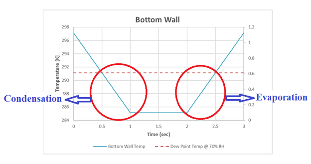
Figure 2.
From the above plot, we can see that the Air volume initial temperature is set to 297.15 K. The Bottom Wall temperature drops to 285.13 K over 1 sec, maintains 285.13 K for 1 sec, and then rises back to 297.15 K over 1 sec. The dew point temperature of the air at 70% RH is 291.14 K and is reached at 0.5 and 2.5 sec. On the whole we can see that both condensation and evaporation occurs when the dew point temperature is reached, as explained above.
Open the HyperMesh Model Database
-
Click the Open Model icon
 located on the standard toolbar.
The Open Model dialog opens.
located on the standard toolbar.
The Open Model dialog opens.
Set the General Simulation Parameters
-
Set the Global Gravity parameters as shown below.
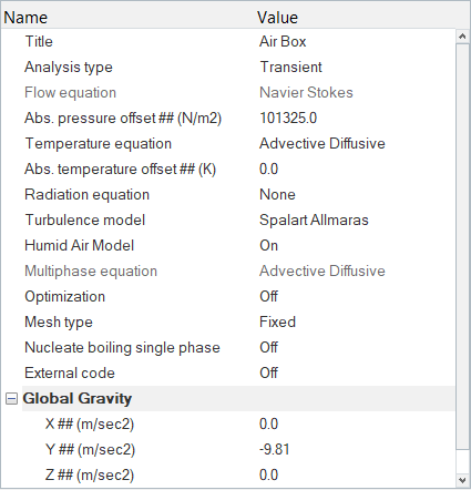
Figure 3. -
Set the Initial time increment to 0.1 and change other
parameters as shown in the figure below.
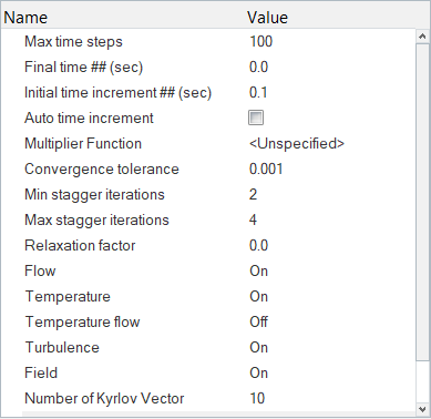
Figure 4.
Set Up Nodal Initial Conditions
-
Change the Default value of Relative Humidity to
70.
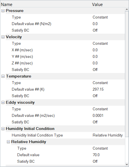
Figure 5.
Set Up Material Model Parameters and Body Force
In this step, you will define the material properties for the problem and assign body force to the fluid volume.
Set Material Model Parameters
-
Enter the values for Density as shown in the figure below and leave the
remaining material parameters unchanged.
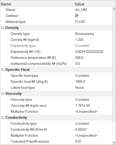
Figure 6. -
Verify that the Material type is set to MULTIPHASE and
the Filed Interaction Type is set to Advective
Diffusive.
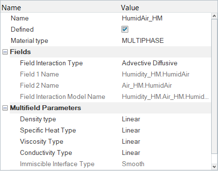
Figure 7.
Set Up Body Force
-
Set Gravity in the Z direction to -9.81.
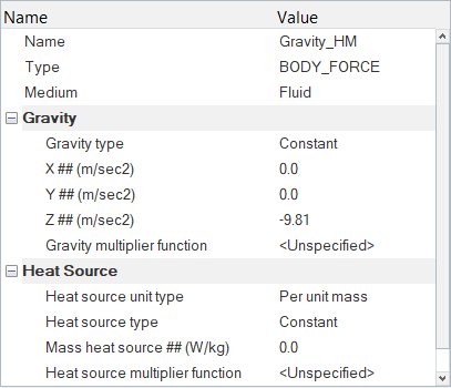
Figure 8.
Create a Multiplier Function
-
In the embedded Entity Editor, change the name to
curve_Temp_MF.
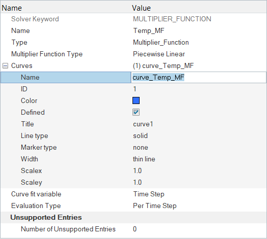
Figure 9. -
Enter the data as shown in the figure below then click
Update in the bottom-left of the window.
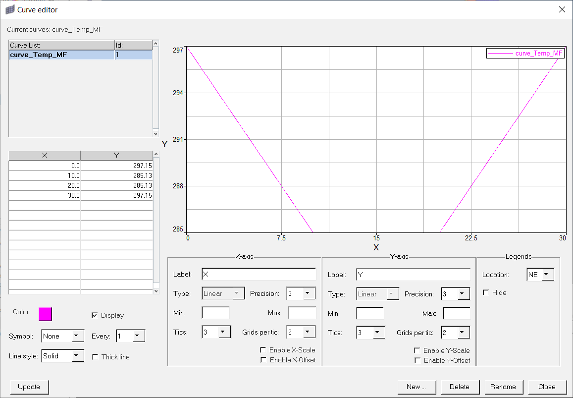
Figure 10.
Set Up Boundary Conditions
-
Click Fluid. In the Entity Editor,
- Set the Type to MULTIPHASE.
- Set the Material to HumidAir_HM.
- Under Element Output, set Active Element Output to On and verify that the other parameters are as shown below.
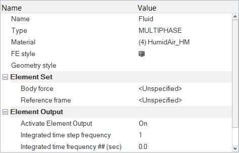
Figure 11. -
Click front. In the Entity Editor, change the Type to SLIP.
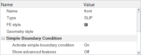
Figure 12. -
Click left. In the Entity Editor,
- Change the Type to WALL.
- Change the Temperature BC type to Flux.
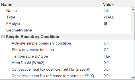
Figure 13. -
Click bottom. In the Entity Editor,
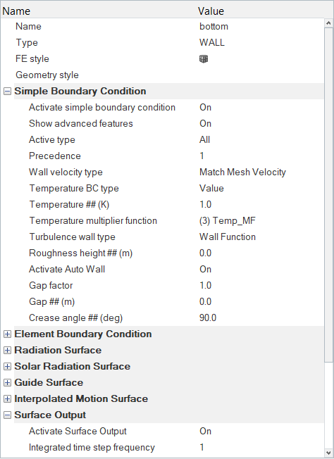
Figure 14.
Set Up Nodal Output Variables
-
Check the box for Output initial condition.
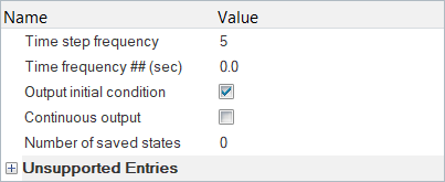
Figure 15.
Compute the Solution
In this step, you will launch AcuSolve directly from HyperMesh and compute the solution.
-
Click
 on the ACU toolbar.
The Solver job Launcher dialog opens.
on the ACU toolbar.
The Solver job Launcher dialog opens. -
Leave the remaining options as
default and click Launch to start the solution
process.
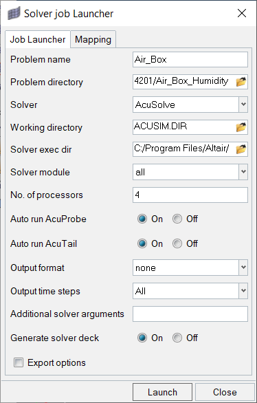
Figure 16.As the solution progresses, an AcuTail and an AcuProbe dialog will open. Solution progress is reported in the AcuTail dialog. An AcuSolve Control dialog will also open from which you can control the solution process. In this dialog you have options to stop the solution or generate the output files at the end of the current time step.A summary of the run printed in the AcuTail dialog indicates that AcuSolve has finished running the solution.
Monitor the Solution with AcuProbe
-
Right-click on Final and select Plot
All.
Note: You might need to click
 on the toolbar in order to
properly display the plot.
on the toolbar in order to
properly display the plot.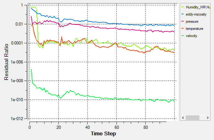
Figure 17. -
Next, expand Relative Humidity then right-click on
relative_humidity and select
Plot.
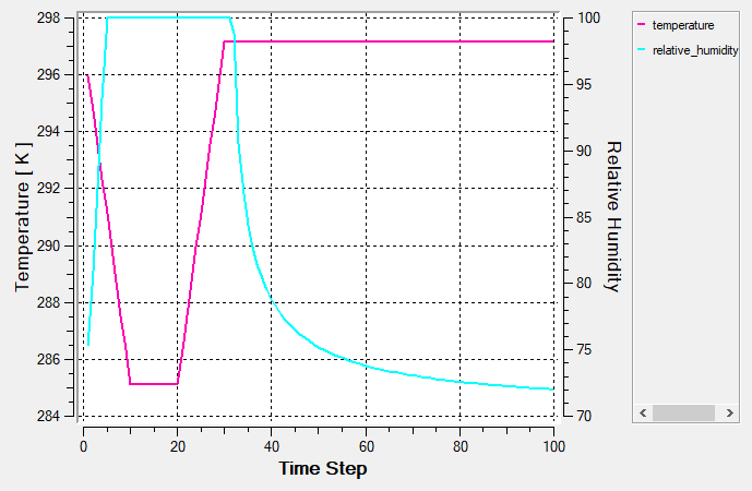
Figure 18. -
Similarly, plot other variables like temperature vs
dewpoint_temperature, as shown in below figure.
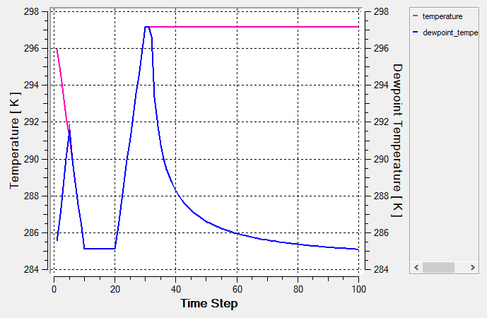
Figure 19. -
Now, plot temperature vs
humidity_film_thickness, as shown in below
figure.
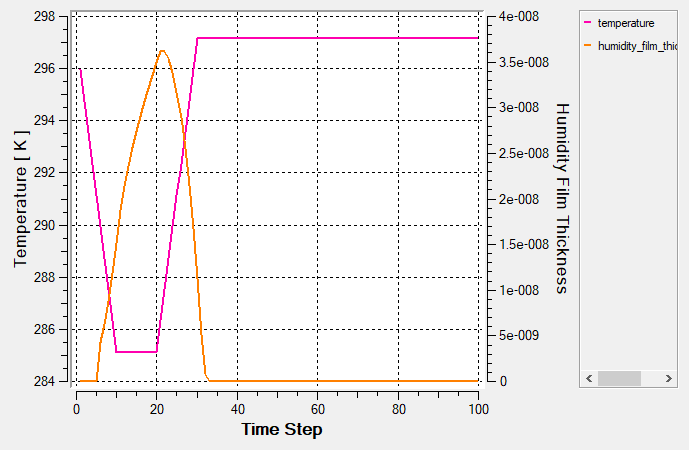
Figure 20. -
Finally, plot relative_humidity vs
humidity_film_thickness, as shown in below
figure.
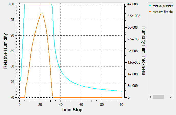
Figure 21.
Post-Process the Results with HyperView
Open HyperView and Load the Model and Results
-
In the Load model and results panel, click
 next
to Load model.
next
to Load model.
-
In the dialog, set the Reader to AcuSolve Result Reader
and Extended nodal output to No.
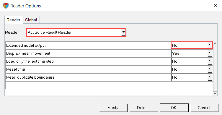
Figure 22.
Create Contours on a Cut Plane
-
Since this is a transient case, you need to plot the results at the last
timestep. To do this, click the Time drop-down menu in the Results Browser and select the last option in the list.
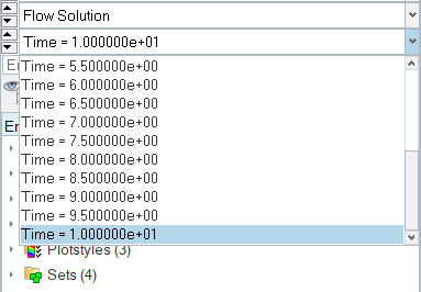
Figure 23.Here we have the last time as 10 sec.
-
Move the Define plane slider bar (located under the Z Axis button) to choose a
desired position for the section cut plane.

Figure 24.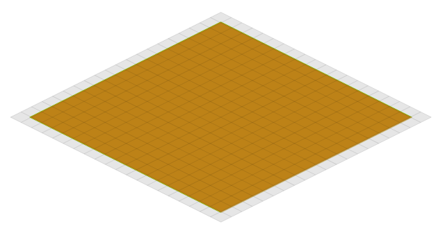
Figure 25. -
Orient the display to the xy-plane by clicking
 on the Standard Views toolbar.
-
Click
 on the Results toolbar to open the Contour panel.
-
Under the Display tab, turn off the Discrete color option.
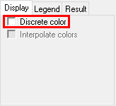
Figure 26.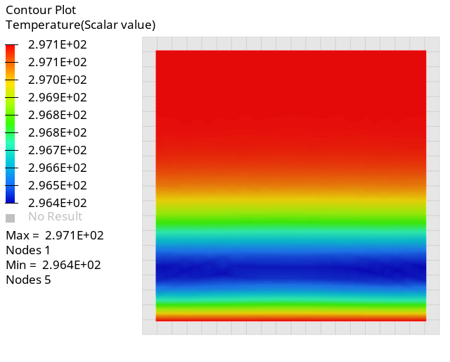
Figure 27. -
Change the Result type to Relative_humidity (s) to view
the relative humidity contour of the XY plane.
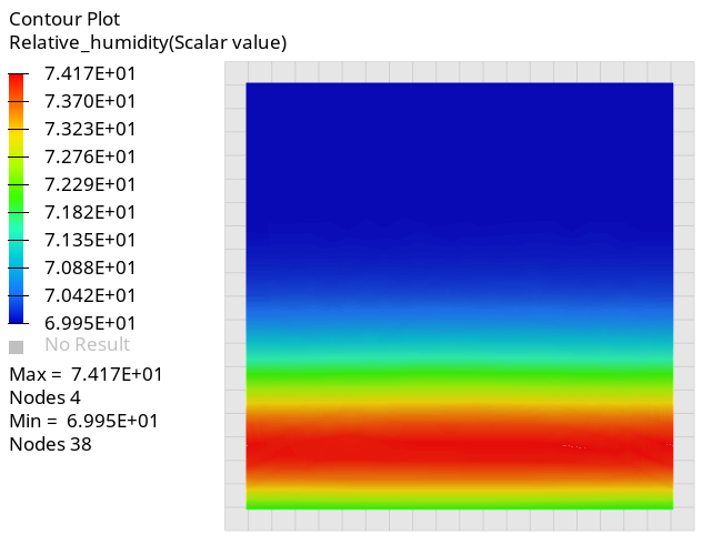
Figure 28. -
Change the Result type to Dew_Point_Temperature (s) to
view the dew point temperature contour of the XY plane.
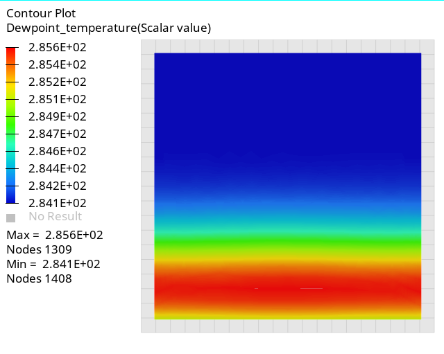
Figure 29. -
Save the plots as an image file.
-
On the Image Capture toolbar, toggle the Save Image
File/Clipboard icon (
 /
/ ) so that it shows .
-
Click the Capture Graphics Area icon
 .
.
-
Provide a name for the image in the dialog then click
Save.
Note: If you wish to use the images in a presentation, you can copy them to the clipboard by toggling the Save Image to File/Clipboard icon to instead of . Then, paste the image in your
presentation.
-
On the Image Capture toolbar, toggle the Save Image
File/Clipboard icon (
Summary
In this tutorial, you worked through a basic workflow to set up and solve a transient multiphase flow problem using HyperMesh and AcuSolve. You also learned how to use the humidity model to quantify accumulation and loss of water vapor on the bottom wall surface due to temperature change. Once the solution was computed, you post-processed the results in HyperView where you created contour plots.