Okumura-Hata Propagation Model
The Okumura-Hata propagation model is a simple empirical model with short computation time.
With this model, only the transmitter and receiver height are processed. The terrain profile between transmitter and receiver is not considered. If, for example, a hill is located between transmitter and receiver, its shadowing effect is not taken into account.
Click and click the Computation tab.
Parameters
- frequency f (150...1500 MHz)
- distance between transmitter and receiver d (1...20 km)
- antenna height of the transmitter (30...200 m)
- antenna height of the receiver (1...10 m)
As the height of the transmitter and the receiver is measured relative to the ground, an effective antenna height ( ) is determined to account for the topographical impact. This also improves the accuracy of the prediction.

Figure 1. Effective antenna height for the Okumura-Hata propagation model.
Settings
- Homogenous environment: For the full prediction area, a homogeneous environment is considered without the settings in the morpho / clutter database.
- Individual environment: As defined in morpho / clutter database.
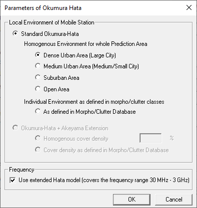
Figure 2. The Parameters of Okumura Hata dialog.
Computation
The following equations show the computation of the basic path loss (in dB) with the model of Hata-Okumura.
- L = path loss (dB)
- f = frequency (MHz)
- Hb = transmitter antenna height above ground (m)
- Hm = receiver antenna height above ground (m)
- d = distance between transmitter and receiver (km)
- a(Hm) = antenna height correction factor
For medium urban area (medium, small city):
For dense urban area (large city):
- f: 150 MHz to 1500 MHz
- Hb: 30 m to 200 m
- Hm: 1 m to 10 m
- d: 1 km to 20 km