Inclusion of the Receiving Antenna
Specify the receiver antenna pattern for a mobile station.

Figure 1. The Consideration of Antenna Properties at Mobile Station group on the Edit Project Parameter dialog - Propagation tab.
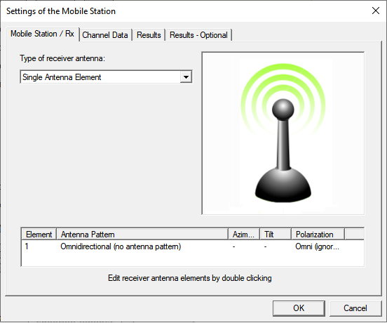
Figure 2. The Settings of the Mobile Station dialog - Mobile Station / Rx tab.
The mobile station is, by default, a single isotropic antenna. With this setting, the received-power result with the mobile station included is the same as for a regular propagation-only simulation, since the propagation-only simulation works with exactly that assumption when calculating the received power. A non-isotropic pattern can be specified by double-left-clicking on Omnidirectional in the table.
Settings of the Mobile Station: Mobile Station / RX Tab
- Single antenna element
- Uniform vertical rectangular antenna array
- Uniform linear antenna array
- Uniform circular antenna array
- Individual location offset for each element
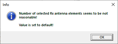
Figure 3. The Info dialog stating that the default value is used.
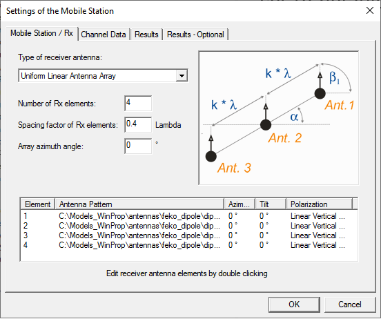
Figure 4. An example of specifying a uniform linear antenna array.
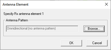
Figure 5. The Antenna Element dialog.
To specify a large antenna array, for example, for massive MIMO, the option Uniform Vertical Rectangular Antenna Array can be used (see Figure 6).
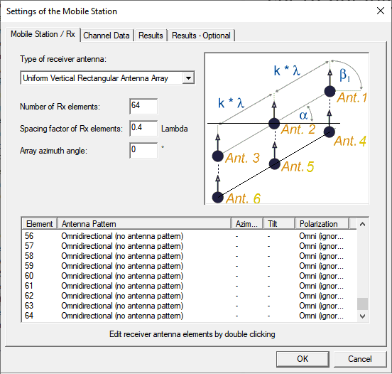
Figure 6. An example of specifying a large antenna array.
The image in Figure 6 has a mixed perspective. The grid of antenna elements is in the vertical plane and is rectangular, with horizontal rows and vertical columns. The angle denotes the rotation of the entire vertical array around the vertical axis (East over North), and the angle denotes the azimuth of the individual antenna elements (East over North).
The image also indicates the numbering, which is row by row. The number of Rx elements is defined in the dialog and then the next integer that is a square is used as a basis. For example, in case of 6 elements defined, a 3x3 vertical array is the basis, and only the antenna elements for the two upper lines are considered. The maximum number of antenna elements is 64, for an 8×8 array.
As the computation of the stream results is very time consuming for larger numbers of elements, the stream results are automatically disabled if more than 4 Tx or Rx elements are defined. However, the subchannel results are computed and written if this option is activated. The memory consumption can become large for simulations with large arrays and many result pixels. Also, the disk usage for the result files can become large.
Settings of the Mobile Station: Channel Data Tab
MIMO systems can be evaluated in more detail by calculating the MIMO channel matrix, which describes the radio channel between each transmit and each receive antenna of the system.
There is a complex single-input-single-output (SISO) channel impulse response of length L+1 between every transmit antenna m and every receive antenna n of a MIMO system.
In this equation, L relates to the tapped delay line, and the time dependence accounts for the possibility that antennas or objects are moving.
The linear time-variant MIMO channel is represented by the channel matrix with dimension :
The MIMO channel matrix can be determined by post-processing the ray data simulation output of a regular propagation simulation by just calculating the phase differences between the single antenna elements of the MIMO antenna arrays at the base station and at the mobile station.
The ray data give a description of all considered propagation paths between the position of the transmitter and each predicted receiver pixel. Field strength, delay and all interaction points (reflections, diffractions, transmissions, scatterings) are listed for the propagation paths that contribute to the signal level at a specified location. Based on these data and the dimensions of the MIMO antenna arrays, the phase shifts between the single elements can be computed in the following way. The transmitter location given in the ray file is assumed to be the center of the transmitting MIMO antenna array. At the receiver side, the same assumption is made. Each point to be computed in area/trajectory/point mode can be assumed to be the center point of a receiving MIMO antenna array. In order to determine the MIMO channel matrix now, only the phase shifts between the single array elements have to be computed, based on the ray data given in the ray file and on the array settings.
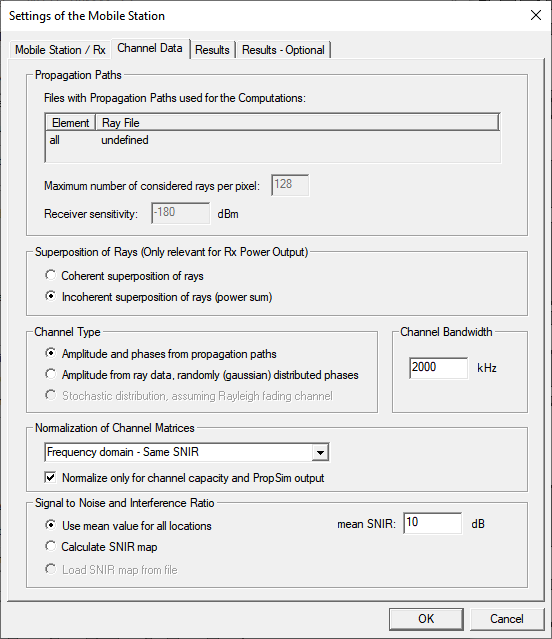
Figure 7. The Settings of the Mobile Station dialog - Channel Data tab.
- Propagation Paths
- The ray data file used for the simulation is listed under Propagation Paths. The maximum number of rays, to be considered for each receiver location is set to 128 (can be only changed manually in the .mic file). This number has to be a power of two. If the ray data file contains more path data for a specific receiver location than specified here, the additional rays are skipped.
- Channel Type
- The radio channels can be modeled using the amplitude and phase information extracted from the ray data file (ray tracing simulation). Alternatively, the phases of the simulated radio channels can be derived randomly, for example, Gaussian distributed random variables are used for the phases. The corresponding amplitudes are taken from the ray tracing simulation. The third option can be used to simulate randomly derived Rayleigh fading channels with statistically distributed amplitudes and phases.
- Channel Bandwidth
-
The bandwidth is considered for the computation of the SNIR (noise power depends on the bandwidth) if the Calculate SNIR map check box is selected.
Furthermore the channel bandwidth is considered for the Frequency Sample Rate (see Results tab).
- Normalization of Channel Matrices
-
The calculated channel matrices can be normalized in various ways using different normalization algorithms either in time or frequency domain. The chosen normalization mode can be applied for all computation steps of the simulation or for the calculation of the MIMO channel capacity and Keysight PROPSIM output only.
The channel capacity of a non-frequency selective MIMO channel can be written as
(4) with the unity matrix I, the overall transmit power P and the noise power. The channel matrices HF have to be determined by NF point Fast Fourier Transformation. The FFT needs to be done for a certain number of sampling points (the number needs to be a power of two) which is by default 128.- Frequency domain - Same path loss
- In order to compare different MIMO channels based on the
same path loss, the system has to be normalized to
fulfil the following condition:where l is the loop index over the sample points in the frequency domain.
(5) - Frequency domain - Same SNIR
- For comparison of different MIMO channels based on the
same SNR, the system has to be normalized to fulfil the
following condition:
(6)
- Signal-to-Noise-and-Interference-Ratio
The signal-to-noise-and-interference-ratio (SNIR) at the receiver locations is used for the calculation of the channel capacity. The SNIR can be specified to be a mean value for all receiver locations. This means the same mean value is considered for all specified receiver locations, independent of the actual received power at the receiver.
The Calculate SNIR map option calculates the SNIR for each receiver location separately taking into account the actual received power as well as the thermal noise (depending on the bandwidth) and an addition interference level, which can be also specified.The Load SNIR map from file option enables the user to load a previously computed SNIR map from the ProMan ray tracing simulation.
Settings of the Mobile Station: Results Tab
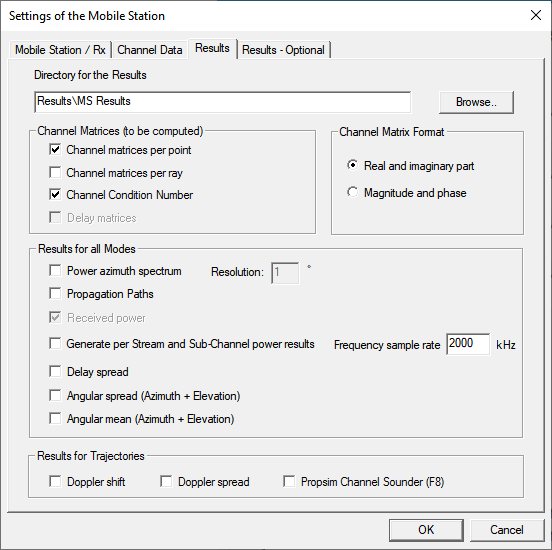
Figure 8. The Settings of the Mobile Station dialog - Results tab.
- Channel Matrices
An overall MIMO channel matrix can be computed per receiver point (Channel matrices per point which is activated by default). This result is derived by summing up coherently all ray contributions impinging on the receiving antenna element. The complex power values of the channel matrices can be written either as real and imaginary part or in amplitude and phase notation.
Additionally, the channel condition number can be computed as well by selecting the Channel Condition Number check box. The MIMO channel condition number is a MIMO performance indicator and computed as ratio of the largest and smallest eigenvalues of the MIMO channel matrix, with lower condition numbers allowing higher data rate transmissions.- Results for all Modes (stationary and non-stationary scenarios)
-
- Generate per stream and sub-channel power results
-
The sub-channel results include the power for a single sub-channel (between one Tx antenna element and one Rx antenna element).
The stream result includes always the best value from the sub-channels (the higher value is always considered without adding anything, as a result, corresponding to selection diversity).
The “normal ” RunMS power result includes the superposition of the sub-channels (for example, power addition in case incoherent superposition has been selected).
- Frequency Sample Rate
- This value is only considered for the ASCII subchannel power results. Defined frequency sample rate is considered together with the defined frequency channel bandwidth (under Channel Data tab) to compute the coherent power superposition for a set of frequency bins, which is done by re-computing the phase of each ray for the new frequency (loop over the frequency bins) and then summing the ray contributions coherently for this frequency bin.
- Results for Trajectories
-
- Doppler shift
- The option Doppler shift gives the Doppler shift per ray due to the velocity along the trajectory in [Hz]. Doppler shift results are only available if the receiver array is moving on a trajectory.
- Doppler spread
- Doppler spread is computed based on the power weighted mean
Doppler shift and represents the square root of the Doppler
variance for all ray contributions (squared difference of
ray Doppler shift minus mean Doppler shift, multiplied with
ray power, normalized with total power (same principle
formulas as for delay spread)).
(7) Doppler spread results are only available if the receiver array is moving on a trajectory.(8) - Propsim Channel Sounder
-
WinProp radio channel data can be converted into the Keysight PROPSIM channel format (.asc file per subchannel and a .shd file).
In order to generate channel data, which can be directly imported into the Keysight PROPSIM F8 channel emulator, some requirements have to be fulfilled:- Calculating the channel data for the channel emulator is only possible for a receiver moving along a trajectory. Therefore a corresponding receiver trajectory must be defined in the ProMan project file and considered in RunPRO. In order to guarantee proper emulation results, the distance resolution should be chosen in such a way, that the resulting evaluation points along the trajectory are located not more than half a wavelength apart from each other. Besides this, the velocity assigned to the defined trajectory points should be constant.
Generating channel data for the Keysight PROPSIM F8 emulator requires channel normalization of type Time Domain - Strongest ray.
Settings of the Mobile Station: Results – Optional Tab
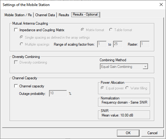
Figure 9. The Settings of the Mobile Station dialog - Results - Optional tab.
- Mutual Antenna Coupling
- This option is disabled by default, as such an analysis is better handled using Altair Feko.
- Diversity Combining
- This option is not available.
- Channel Capacity
- The ergodic and / or outage MIMO channel capacity is computed by calculating the eigenvalues for equal power or water filling power allocation mode. The results are available for each specified receiver location as well as in terms of probability density functions and cumulated probability density functions. The chosen normalization mode for the channel matrices and the considered SNIR (defined on the Channel Configuration dialog) are displayed here as these settings have a strong influence on the channel capacity.
After Specifying the Mobile Station
- Click .
- Click the
 RunMS icon in the project toolbar.
 - Press F6 to use the keyboard shortcut.
- RunPro
- RunMS
- RunNet
Of the three simulation types, the propagation simulation (RunPro) tends to be the most time consuming. Sometimes you need to modify the properties of the mobile station, or modify related output requests, without losing the results of the regular propagation simulation. That can be achieved by accessing .
This option is not available (grayed out) in a new project. It becomes available when the Consider Antenna of MS check box was selected ( - Propagation tab.