System Configuration
Configure the wireless system to be simulated using the System Configuration dialog.
The wireless system to be simulated can be configured via in the Project menu or by clicking the corresponding button of the Project toolbar.
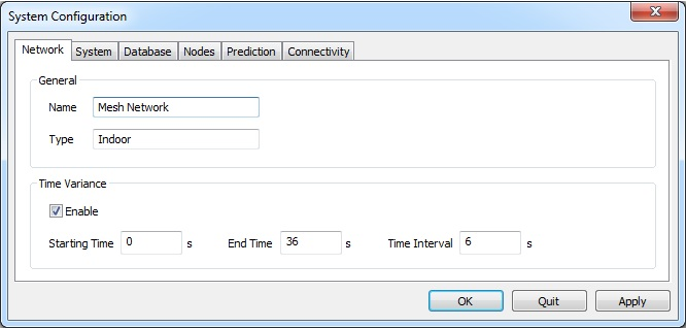
Figure 1. The System Configuration dialog showing the Network tab.
Network Tab
On the Network tab you can set general definitions for the overall network.
- General
- General network settings:
- Time Variance
- Available for indoor projects. Node locations and orientations as well as objects
of the vector database can vary over time.
- Enable
- Enable or disable time variance for whole project.
- Starting time
- First time stamp of simulation in seconds.
- End time
- Last time stamp of simulation in seconds.
- Time interval
- Granularity of time stamps between starting time and end time in seconds. For example, a starting time of 0 seconds, an end time of 10 seconds and a time interval of 1 second result in 11 time stamps with a time difference of 1 second.
System Tab
On the System tab you can set parameters that define the wireless air interface.
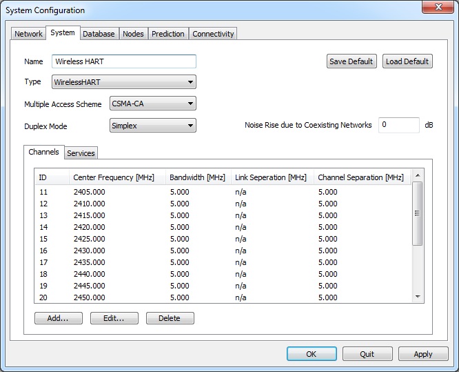
Figure 2. The System Configuration dialog showing the System tab.
- Name
- Arbitrary name to identify the wireless system.
- Save Default / Load Default
- Save current system configuration to the Component Catalog or load a system configuration from the Component Catalog, respectively.
- Type
- Type of air interface. This parameter can not be changed in CoMan
- Multiple Access Scheme
- Multiple access scheme of the air interface. This parameter is typically set to CSMA-CA (carrier sense multiple access with collision avoidance) for mesh/sensor networks.
- Duplex Mode
- The duplex mode of the system is automatically pre-selected depending on the chosen multiple access system but can also be changed manually.
- Noise Rise due to Coexisting Networks
- Coexisting networks operating in the same or in adjacent frequency bands cause additional interference, which can be specified here.
- Channels
- The available radio channels of the system are listed on the Channels tab. Channel Configurations can be added, modified or deleted using the Add, Edit, and Delete buttons.
- Services
- The available services of the wireless system can be defined on the Services tab of the dialog page. At least one service has to be defined per system. Service Configurations can be added, modified or deleted using the Add, Edit, and Delete buttons.
Database Tab
The databases used for the simulations are listed on the Database tab. Depending on the project different types of databases (vector, topography, clutter) are available.
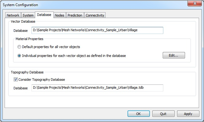
Figure 3. The System Configuration dialog showing the Database tab.
- Vector Database
- Available for indoor and urban projects.
- Topography Database
- Available for urban (optional) and rural projects.
- Consider Topography Database
- For urban projects, the consideration of topography database (if available) is optional and can be disabled. The topography database is mandatory for rural projects and must be considered
- Database
- Path and file name of the topography database.
Nodes Tab
All nodes of the network are listed on the Nodes tab. Node Configurations can be added, modified or deleted by pressing the corresponding buttons at the bottom of the dialog. Configuration of Multiple Nodes/Transceivers is possible if multiple nodes are selected before pressing the Edit button.
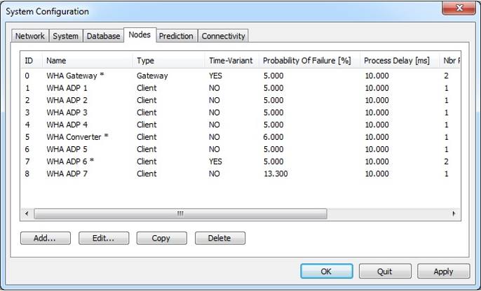
Figure 4. The System Configuration dialog showing the Nodes tab.
Prediction Tab
The parameters of the simulation area and the wave propagation model can be specified on the Prediction tab. Wave propagation results can be selected in the lower section of the dialog.
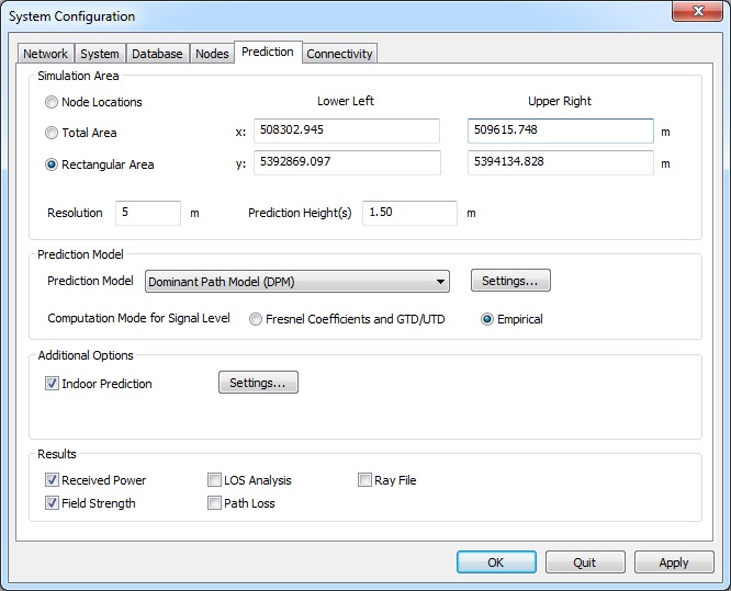
Figure 5. The System Configuration dialog showing the Prediction tab.
- Simulation Area
- Wave propagation results can be computed at the locations of the nodes
(point-to-point prediction), for the total available simulation area or for an
arbitrary rectangular area smaller than the total simulation area. The
point-to-point prediction for the locations of the nodes is required for the
simulation of the connectivity between the nodes.
- Resolution
- Specify the resolution (pixel size) of the propagation results.Note: The smaller the resolution, the more accurate the prediction results. However, the computation time increases with decreasing resolution of the prediction area.
- Prediction Height(s)
- Prediction heights can be specified for area predictions only. Multiple prediction heights can be defined in indoor environments only and have to be separated with spaces.
- Prediction Model
- The available prediction models suitable for the chosen simulation environment
are listed in the drop-down list. The settings of the selected
propagation model can be edited by clicking on the Settings
button. Note: The point-to-point prediction mode for predictions at node locations is supported for only a subset of the available propagation models.
- Computation Mode for Signal Level
-
The computation mode for the signal level along the propagation path can be either deterministic (Fresnel Coefficients and GTD/UTD) or Empirical. The deterministic mode uses Fresnel Equations for the determination of the reflection and transmission loss and the GTD/UTD for the determination of the diffraction loss. This model has a slightly longer computation time and uses three physical material parameters (permittivity, permeability and conductivity). The empirical mode uses five empirical material parameters (minimum loss of incident ray, maximum loss of incident ray, loss of diffracted ray, reflection loss, transmission loss).
For correction purposes or for the adaptation to measurements, an offset to those material parameters can be specified. As a result, the empirical model has the advantage that the needed material properties are easier to obtain than the physical parameters required for the deterministic model. Also the parameters of the empirical model can more easily be calibrated with measurements. It is therefore easier to achieve a high accuracy with the empirical model.
Note: Please refer to the ProMan user manual for more details about the wave propagation models.
- Additional Options
- For urban environments indoor predictions of the buildings can also be done. Settings of the Optional Indoor Prediction can be specified by clicking on the Settings... button after enabling the Indoor Prediction option.
- Results
- Results which shall be computed and saved to disk during wave propagation simulation can be enabled or disabled.
Connectivity
Additional parameters for connectivity simulations can be specified on the Connectivity tab.
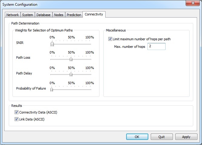
Figure 6. The System Configuration dialog showing the Connectivity tab.
- Path determination
-
- Weights for Selection of Optimum Paths
- The path searching algorithm uses four values
(signal-to-noise-and-interference ratio at the receiving node, path loss
between two nodes, path delay between two nodes and probability of
failure along the path between two nodes) to determine the optimum path
of information flow between the nodes of the network. The effects of the
different values (weight factors) can be defined to be between zero and
one hundred percent each.Note: Along a path containing more than two nodes, the maximum SNIR value and the maximum path loss value occurring along the path is considered, whereas the values of path delay and probability of failure are summed up along the path.
- Miscellaneous
- The maximum number of hops per path, i.e. the maximum number of nodes between transmitter and receiver node can be limited optionally. This makes it possible to configure the path determination according to the limitations of the hardware.
- Results
- Results which shall be computed and saved to disk during connectivity simulation can be enabled or disabled.