Comparison of Wave Propagation Results for Tx Height of 10m
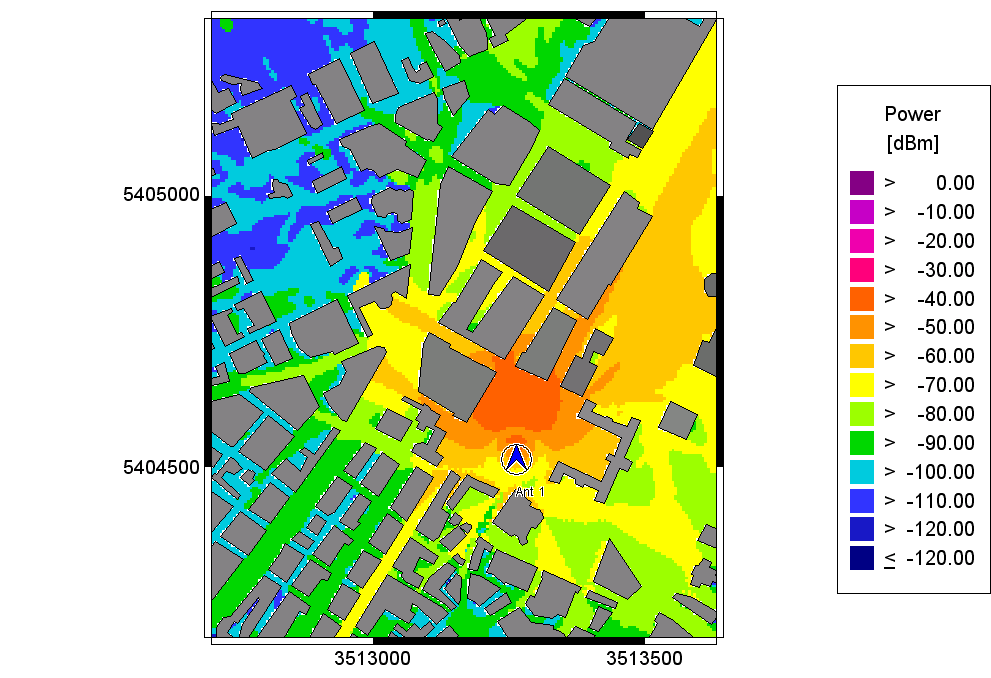
Figure 1. Prediction of received power using the measured 3D antenna pattern (Tx height 10 m).
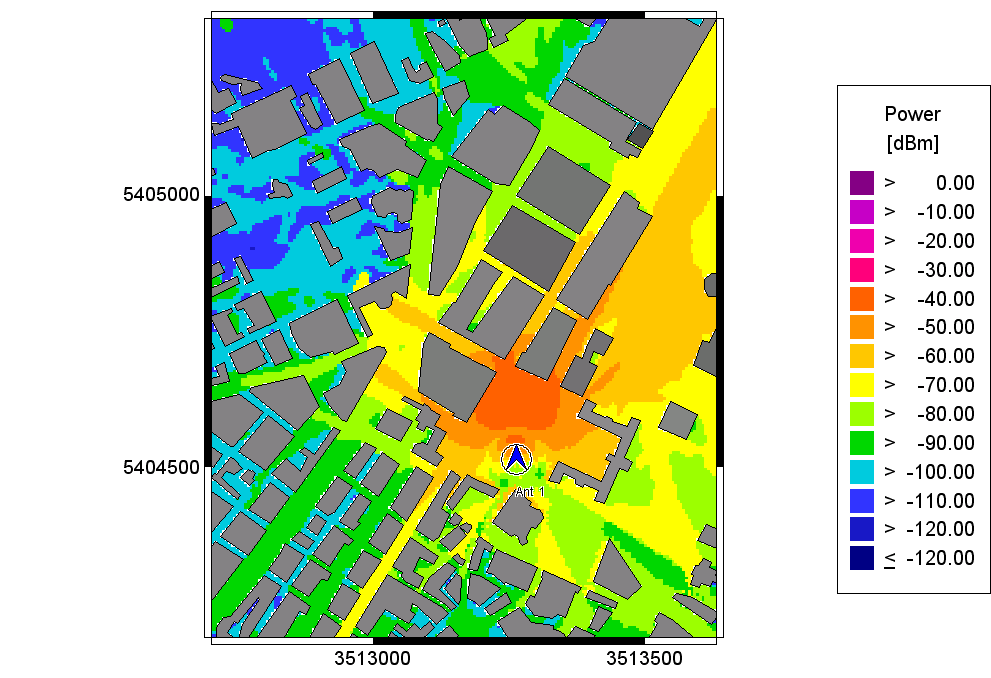
Figure 2. Prediction of received power using the interpolated 3D pattern (AM algorithm).
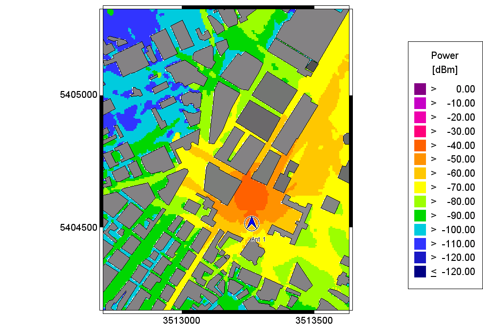
Figure 3. Prediction of received power using the interpolated 3D pattern (BI algorithm).
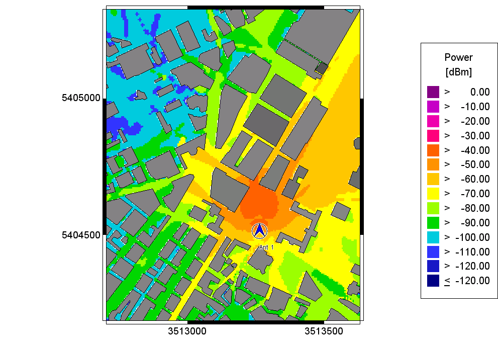
Figure 4. Prediction of received power using the interpolated 3D pattern (WBI algorithm).
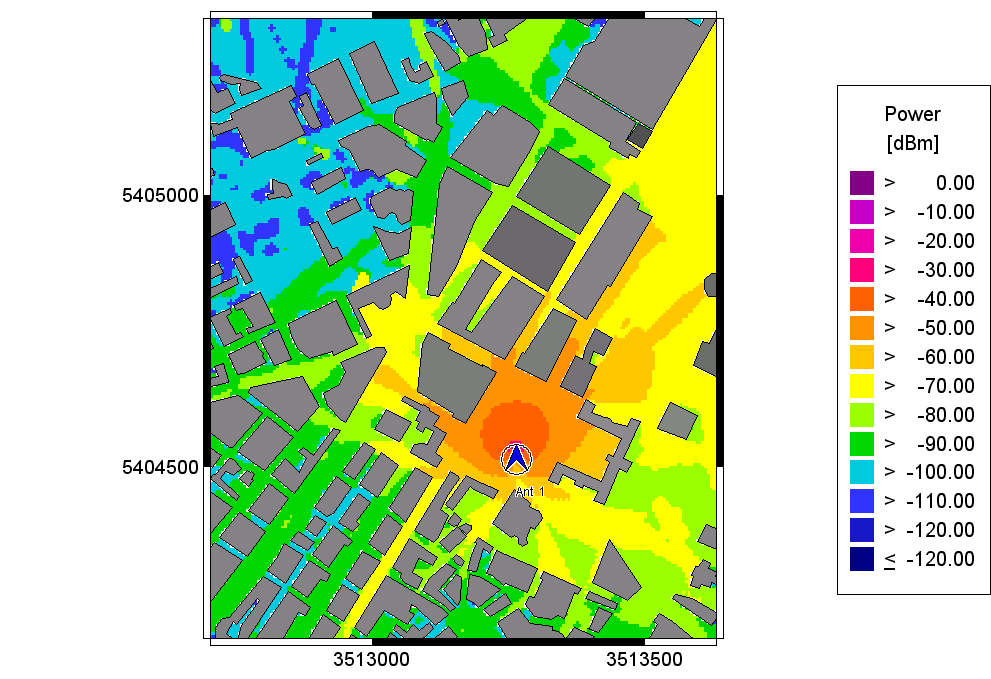
Figure 5. Prediction of received power using the interpolated 3D pattern (HPI algorithm).
The plots of the predicted received power for the transmitter height of 10m show the influence of the antenna pattern on the wave propagation computation. Also for this reduced transmitter height, all the figures look very similar, however after detailed analysis, there are some differences visible.
| Comparison | Polarization +45° | Polarization -45° | ||
|---|---|---|---|---|
| Measured 3D Pattern | Mean Value [dB] | Standard Deviation [dB] | Mean Value [dB] | Standard Deviation [dB] |
| AM algorithm | 0.19 | 1.58 | 0.07 | 0.78 |
| BI algorithm | -0.72 | 1.71 | -1.43 | 2.21 |
| WBI algorithm | -1.68 | 1.84 | -2.06 | 1.85 |
| HPI algorithm | -0.23 | 1.41 | -0.34 | 1.11 |
The numerical evaluation of these differences is listed in the table above. According to this evaluation, the AM algorithm has the best performance (the smallest error with respect to the measured 3D antenna pattern). However, the HPI algorithm achieves nearly the same performance.