GTCMAT
Utility/Data Access SubroutineGTCMAT calculates the compliance matrix between "N" REFERENCE_MARKERs in a MotionSolve model.
Use
GTCMAT is usually called from a REQSUB user subroutine.
Format
- Fortran Calling Syntax
- CALL GTCMAT (NM, MKID, NC, CMAT, ISTAT)
- C/C++ Calling Syntax
- c_gtcmat(nm, mkid, nc, cmat, istat)
- Python Calling Syntax
- [cmat, istat] = py_gtcmat(mkid)
Attributes
- NM
- Integer
- MKID
- Integer
- NC
- Integer
Output
- CMAT
- Double Precision
- ISTAT
- Integer
Examples
| Units | Properties | Geometry |
|---|---|---|
| Length = mm Mass = Kg Time = Seconds Force = Newtons |
Mass properties of T mass = 170.1587874 Kg inertia = 1.607495985E+007, 1.181530722E+007, 4.33055212E+006 Stiffness characteristics at B1, B2 and B3: K = 200, 200, 200 KT = 2.291831181E+005, 2.864788976E+005, 3.437746771E+005 |
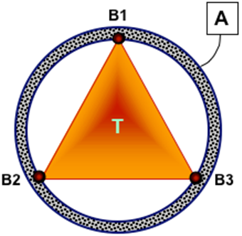 Figure 1. A Triangle T Suspended from an Annulus A |
A REQSUB is written to calculate the compliance matrix. In the REQSUB, GTCMAT is invoked with the appropriate parameters. The REQSUB obtains the compliance matrix and writes it to a file. The contents of this file are shown below.
The file contains an 18 by 18 matrix, conveniently partitioned into 6 by 6 blocks.
COMPLIANCE MATRIX
=================
IM = B1 JM = B1
Row Range =  1 -- 6
Col Range =  1 -- 6
    2.78486E-03    0.00000E+00    0.00000E+00    0.00000E+00    0.00000E+00   -2.79544E-06
    0.00000E+00    1.66667E-03    0.00000E+00    0.00000E+00    0.00000E+00    0.00000E+00
    0.00000E+00    0.00000E+00    3.49751E-03    4.57714E-06    0.00000E+00    0.00000E+00
    0.00000E+00    0.00000E+00    4.57711E-06    0.00000E+00    0.00000E+00    0.00000E+00
    0.00000E+00    0.00000E+00    0.00000E+00    0.00000E+00    0.00000E+00    0.00000E+00
   -2.79548E-06    0.00000E+00    0.00000E+00    0.00000E+00    0.00000E+00    0.00000E+00
IM = B1 JM = B2
Row Range =  1 -- 6
Col Range =  7 --12
    1.10757E-03    8.38643E-04    0.00000E+00    0.00000E+00    0.00000E+00   -2.79544E-06
    0.00000E+00    1.66667E-03    0.00000E+00    0.00000E+00    0.00000E+00    0.00000E+00
    0.00000E+00    0.00000E+00    7.51245E-04    4.57714E-06    0.00000E+00    0.00000E+00
    0.00000E+00    0.00000E+00   -2.28855E-06    0.00000E+00    0.00000E+00    0.00000E+00
    0.00000E+00    0.00000E+00    3.51939E-06    0.00000E+00    0.00000E+00    0.00000E+00
    1.39774E-06   -2.09661E-06    0.00000E+00    0.00000E+00    0.00000E+00    0.00000E+00
IM = B1 JM = B3
Row Range =  1 -- 6
Col Range = 13 --18
    1.10757E-03   -8.38643E-04    0.00000E+00    0.00000E+00    0.00000E+00   -2.79543E-06
    0.00000E+00    1.66667E-03    0.00000E+00    0.00000E+00    0.00000E+00    0.00000E+00
    0.00000E+00    0.00000E+00    7.51245E-04    4.57714E-06    0.00000E+00    0.00000E+00
    0.00000E+00    0.00000E+00   -2.28855E-06    0.00000E+00    0.00000E+00    0.00000E+00
    0.00000E+00    0.00000E+00   -3.51939E-06    0.00000E+00    0.00000E+00    0.00000E+00
    1.39774E-06    2.09661E-06    0.00000E+00    0.00000E+00    0.00000E+00    0.00000E+00
IM = B2 JM = B1
Row Range =  7 --12
Col Range =  1 -- 6
    1.10757E-03    0.00000E+00    0.00000E+00    0.00000E+00    0.00000E+00    1.39772E-06
    8.38643E-04    1.66667E-03    0.00000E+00    0.00000E+00    0.00000E+00   -2.09658E-06
    0.00000E+00    0.00000E+00    7.51245E-04   -2.28857E-06    3.51938E-06    0.00000E+00
    0.00000E+00    0.00000E+00    4.57711E-06    0.00000E+00    0.00000E+00    0.00000E+00
    0.00000E+00    0.00000E+00    0.00000E+00    0.00000E+00    0.00000E+00    0.00000E+00
   -2.79548E-06    0.00000E+00    0.00000E+00    0.00000E+00    0.00000E+00    0.00000E+00
IM = B2 JM = B2
Row Range =  7 --12
Col Range =  7 --12
    1.94621E-03   -4.19322E-04    0.00000E+00    0.00000E+00    0.00000E+00    1.39772E-06
   -4.19322E-04    2.29565E-03    0.00000E+00    0.00000E+00    0.00000E+00   -2.09658E-06
    0.00000E+00    0.00000E+00    3.18019E-03   -2.28857E-06    3.51938E-06    0.00000E+00
    0.00000E+00    0.00000E+00   -2.28855E-06    0.00000E+00    0.00000E+00    0.00000E+00
    0.00000E+00    0.00000E+00    3.51939E-06    0.00000E+00    0.00000E+00    0.00000E+00
    1.39774E-06   -2.09661E-06    0.00000E+00    0.00000E+00    0.00000E+00    0.00000E+00
IM = B2 JM = B3
Row Range =  7 --12
Col Range = 13 --18
    1.94621E-03    4.19322E-04    0.00000E+00    0.00000E+00    0.00000E+00    1.39772E-06
   -4.19322E-04    1.03768E-03    0.00000E+00    0.00000E+00    0.00000E+00   -2.09658E-06
    0.00000E+00    0.00000E+00    1.06856E-03   -2.28857E-06    3.51938E-06    0.00000E+00
    0.00000E+00    0.00000E+00   -2.28855E-06    0.00000E+00    0.00000E+00    0.00000E+00
    0.00000E+00    0.00000E+00   -3.51939E-06    0.00000E+00    0.00000E+00    0.00000E+00
    1.39774E-06    2.09661E-06    0.00000E+00    0.00000E+00    0.00000E+00    0.00000E+00
IM = B3 JM = B1
Row Range = 13 --18
Col Range =  1 -- 6
    1.10757E-03    0.00000E+00    0.00000E+00    0.00000E+00    0.00000E+00    1.39772E-06
   -8.38643E-04    1.66667E-03    0.00000E+00    0.00000E+00    0.00000E+00    2.09658E-06
    0.00000E+00    0.00000E+00    7.51245E-04   -2.28857E-06   -3.51938E-06    0.00000E+00
    0.00000E+00    0.00000E+00    4.57711E-06    0.00000E+00    0.00000E+00    0.00000E+00
    0.00000E+00    0.00000E+00    0.00000E+00    0.00000E+00    0.00000E+00    0.00000E+00
   -2.79548E-06    0.00000E+00    0.00000E+00    0.00000E+00    0.00000E+00    0.00000E+00
IM = B3 JM = B2
Row Range = 13 --18
Col Range =  7 --12
    1.94621E-03   -4.19322E-04    0.00000E+00    0.00000E+00    0.00000E+00    1.39772E-06
    4.19322E-04    1.03768E-03    0.00000E+00    0.00000E+00    0.00000E+00    2.09658E-06
    0.00000E+00    0.00000E+00    1.06856E-03   -2.28857E-06   -3.51938E-06    0.00000E+00
    0.00000E+00    0.00000E+00   -2.28855E-06    0.00000E+00    0.00000E+00    0.00000E+00
    0.00000E+00    0.00000E+00    3.51939E-06    0.00000E+00    0.00000E+00    0.00000E+00
    1.39774E-06   -2.09661E-06    0.00000E+00    0.00000E+00    0.00000E+00    0.00000E+00
IM = B3 JM = B3
Row Range = 13 --18
Col Range = 13 --18
    1.94621E-03    4.19322E-04    0.00000E+00    0.00000E+00    0.00000E+00    1.39772E-06
    4.19322E-04    2.29565E-03    0.00000E+00    0.00000E+00    0.00000E+00    2.09658E-06
    0.00000E+00    0.00000E+00    3.18019E-03   -2.28857E-06   -3.51938E-06    0.00000E+00
    0.00000E+00    0.00000E+00   -2.28855E-06    0.00000E+00    0.00000E+00    0.00000E+00
    0.00000E+00    0.00000E+00   -3.51939E-06    0.00000E+00    0.00000E+00    0.00000E+00
    1.39774E-06    2.09661E-06    0.00000E+00    0.00000E+00    0.00000E+00    0.00000E+00
The 18x18 matrix is organized in 6x6 blocks as shown below. Blocks that are transposes of each other are shaded in the same color.
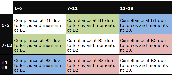
Figure 2. Black definition in the compliance matrix, CMAT.
Comments
- GTCMAT is called from a user-written subroutine. GTCMAT must be called when IFLAG = TRUE in the user subroutine from which it is called.
- The compliance matrix is a transfer function for a system
calculated at static equilibrium. A transfer function requires inputs and outputs.
For a compliance matrix calculation, these are defined as follows:
- represents the inputs to the linearized system. It is an array of size 6*NM. Each component is a force or torque acting in one of the six directions at the "NM" REFERENCE_MARKERs.
- represents the outputs from the linearized system. It is an array of dimension 6*NM. Each component is a translational or rotational displacement acting in one of the six directions at the "NM" REFERENCE_MARKERs.
- At static equilibrium, the transfer function
of a system with inputs
and
outputs may be represented as:
(1) The quantities in the above equation are defined as follows:- represents the Laplace domain variable. is the damping, is the frequency of the vibration state, and is .
- are constant valued matrices of appropriate dimension. They are called the state matrices for the system at the operating point.
- is a 6NM x 6NM matrix.
- For the ith
REFERENCE_MARKER of interest, I, in the system, the six inputs
are defined as follows:
- A unit force at the origin of I, acting along the x-axis of the global coordinate system.
- A unit force at the origin of I, acting along the y-axis of the global coordinate system.
- A unit force at the origin of I, acting along the z-axis of the global coordinate system.
- A unit torque on I, acting about the x-axis of the global coordinate system.
- A unit torque on I, acting about the y-axis of the global coordinate system.
- A unit torque on I, acting about the z-axis of the global coordinate system.
- For the jth
REFERENCE_MARKER of interest, J, in the system, the outputs are
defined as follows:
- The translational displacement of the origin of J measured along the x-axis of the global coordinate system, due to an input .
- The translational displacement of the origin of J measured along the y-axis of the global coordinate system, due to an input .
- The translational displacement of the origin of J measured along the z-axis of the global coordinate system, due to an input .
- The small angle approximation of the rotation of J, due to input , measured about the x-axis of the global coordinate system.
- The small angle approximation of the rotation of J, due to input , measured about the y-axis of the global coordinate system.
- The small angle approximation of the rotation of J, due to input , measured about the y-axis of the global coordinate system.
- Compliance matrix calculation is
particularly useful in suspension elasto-kinematic evaluations. Several suspension
design factors can be expressed as a function of quantities in the compliance
matrix.
For example, the vertical wheel rate is defined as the inverse of the vertical displacement measures at the wheel center, due to a vertical load applied at the wheel center.
Assuming that the compliance matrix between two markers located at the suspension wheel center has been computed, then it is quite obvious to express the vertical wheel rate as follows:
- Left vertical wheel rate =
- Right vertical wheel rate =
Where the various terms are entries in the compliance matrix are:
- = vertical displacement of the left wheel due to a unit vertical force applied to the left wheel.
- = vertical displacement of the left wheel due to a unit vertical force applied to the right wheel.
- = vertical displacement of the right wheel due to a unit vertical force applied to the left wheel.
- = vertical displacement of the right wheel due to a unit vertical force applied to the right wheel.
- Another typical compliance matrix application is the calculation of motion ratios for springs and dampers. Spring motion ratio is defined as the ratio between the relative displacement along the axis of the spring and the relative load applied between the upper and lower spring seats. This quantity can be easily obtained by computing the compliance matrix between a marker positioned at the lower spring seat and a marker positioned at the upper spring seat.