Multipole Array Simulation
This example shows how to simulate an array of dipoles and how to create the multipole file and how to use it in another project.
Step 1: Create a new MOM Project.
Open newFASANT and select 'File --> New' option.
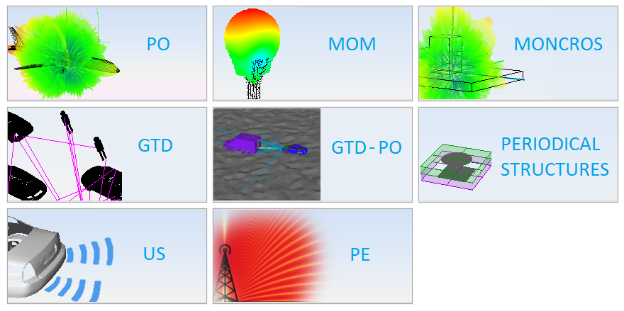
Select 'MOM' option on the previous figure and start to configure the project.
Step 2: Set Simulation Parameters
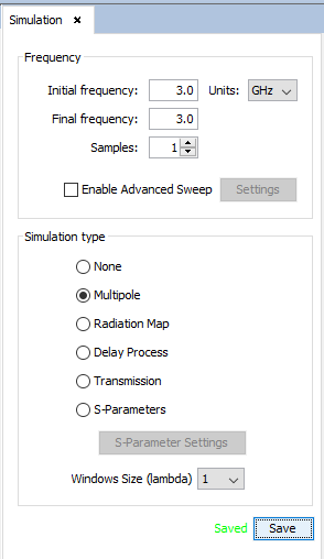
Select 'Simulation --> Parameters' option on the menu bar and the following panel appears. Set up the frequency at 3 GHz and the multipole option, as the next figure shows and save it.
Step 3: Set the source parameters. To obtain more information about sources and antennas see Antennas.
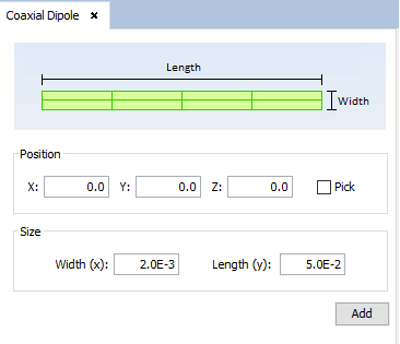
In this example, a physical dipole (coaxial feed) is set up.
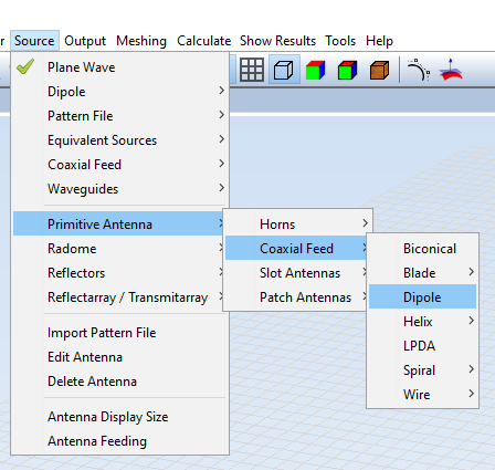
Select 'Antenna --> ‘Primitive Antenna’ --> ‘Coaxial Feed’ --> ‘Dipole' option and set the parameters as show the next figure. Then save the parameters and the dipole appears.
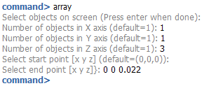
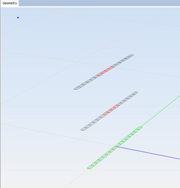
Step 4: Using the array command, a small array is created.
Step 5: Create the geometry model. To obtain more information about geometries generation see Geometry Menu.
Execute 'box' command writing it on the command line and sets the parameters as the next figure shows when command line ask for it.
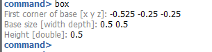
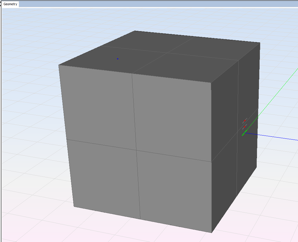
Note if you are doing this example to obtain the multipole file (arraySmallBoxMultipole4lambda.suj) to be used on (GTD-Example) then, to get a faster simulation, the dimensions of the box are:
First point -0.225, -0.1, -0.1
Width 0.2
Depth 0.2
Height 0.2
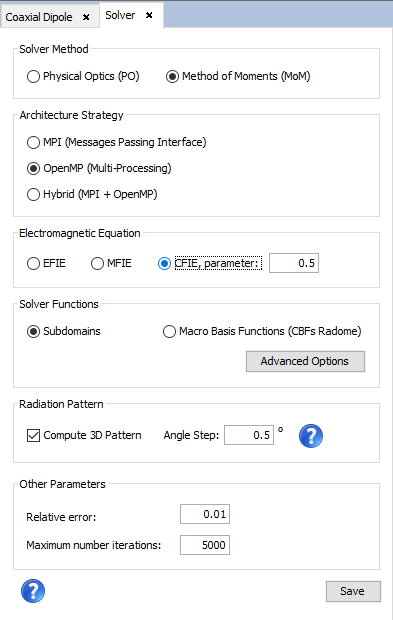
Step 6: Solver parameters menu.
As you can see in the below figure, in this example, CFIE is setting up.
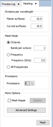
Step 7: Meshing the geometry model.
Select 'Meshing --> Parameters' to open the meshing configuration panel and then set the parameters as show the next figure. In order to obtain the shortest possible time for meshing, it is recommended to run the process of meshing with the number of physical processors available to the machine.
Step 8: Execute the simulation. In order to obtain the shortest possible time for calculating the results, it is recommended to run the process with the number of physical processors available to the machine.
Select 'Calculate --> Execute' option to open simulation parameters.
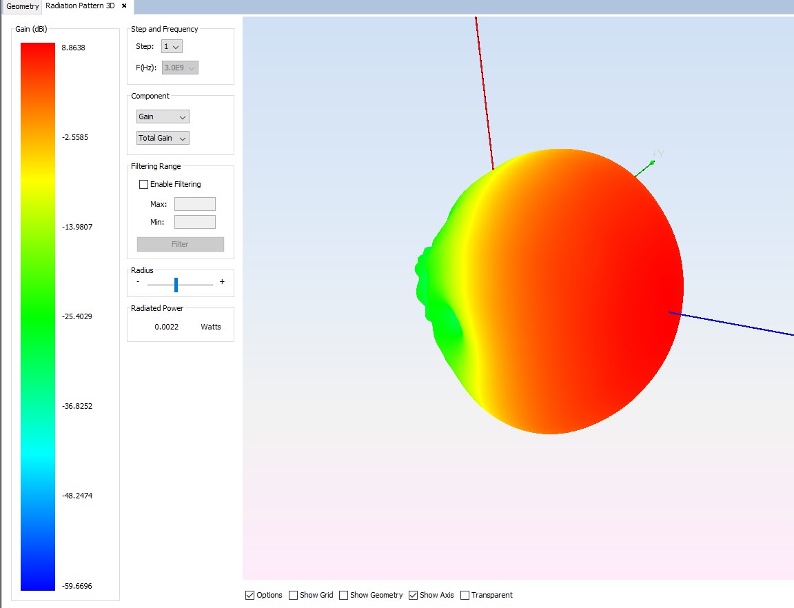
Step 9: Show Results. To get more information about the graphics panel advanced options (clicking on the right button of the mouse over the panel) see Annex 1: Graphics Advanced Options.
Select 'Show Results --> Radiation Pattern --> View 3D Pattern' option to show the cuts of the radiation pattern options.
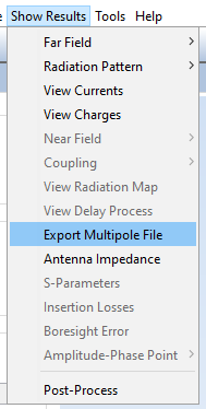
Step 10: Export Multipole File.
Select 'Show Results --> Export Multipole File' option to save the multipole file on a selected path for use in other simulations. Previous, select the step and frequency for the multipole file.
Step 11: Close the project and open a new MoM Project.
In the new project, we import the previously created multipole. Because the geometry in the previous project is very big we have many multipole, each multipole model the radiation of the current in each cube of one wavelength of side. We can use this multipole to compute the fields at a distance greater than 2*(D**2)/lambda, where D is the size of the cubes. In this case this distance is given by 2*(lambda**2)/lambda = 2*lambda= 20 cm.
The process to create this project is similar to the previous one, the main changes are on the next steps:
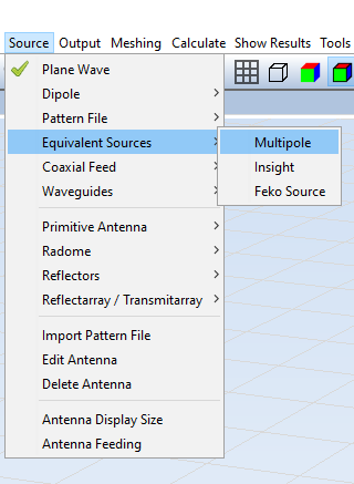
Step 1: Set the source parameters. To obtain more information about sources and antennas see Antennas.
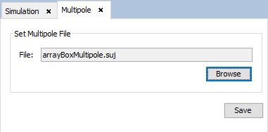
Select 'Antenna --> ‘Primitive Antenna’ --> ‘Equivalent Sources’ --> ‘Multipole' option and set the parameters as show the next figure. Then save the parameters and the dipole appears.
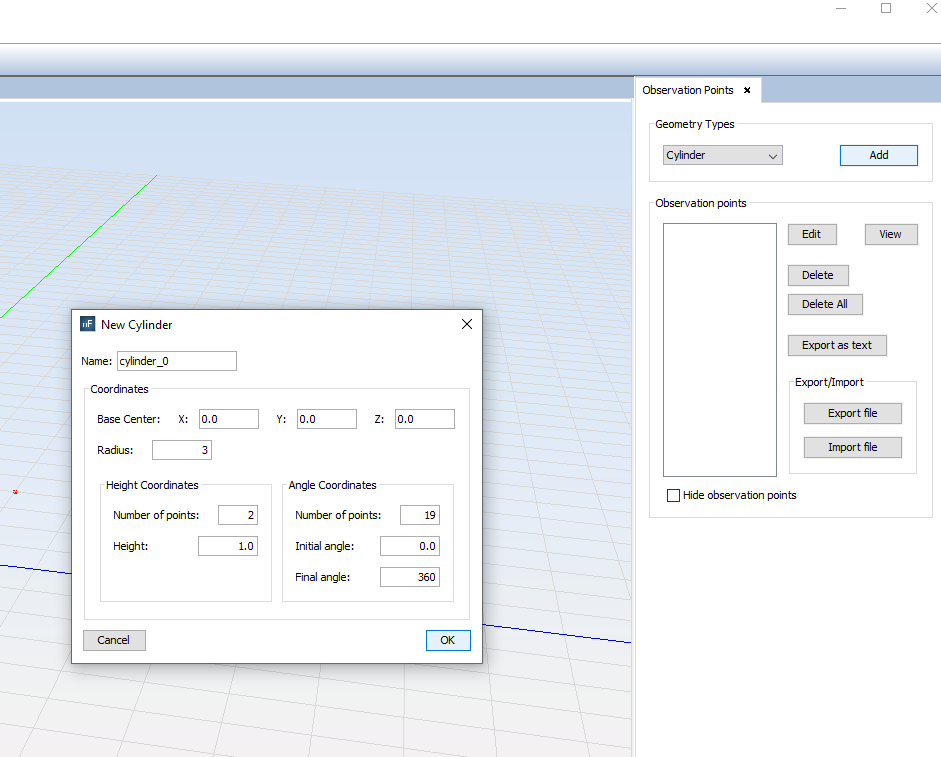
Step 2: Set Near Field Parameters
Select ‘Output’ --> ‘Observation Points’ option. Select ‘cylinder’ on the selector ‘Geometry Types’ section and click on ‘Add’ button. The line parameters panel will appear, then set up the values as the next figure show and accept it clicking on ‘Ok’ button.
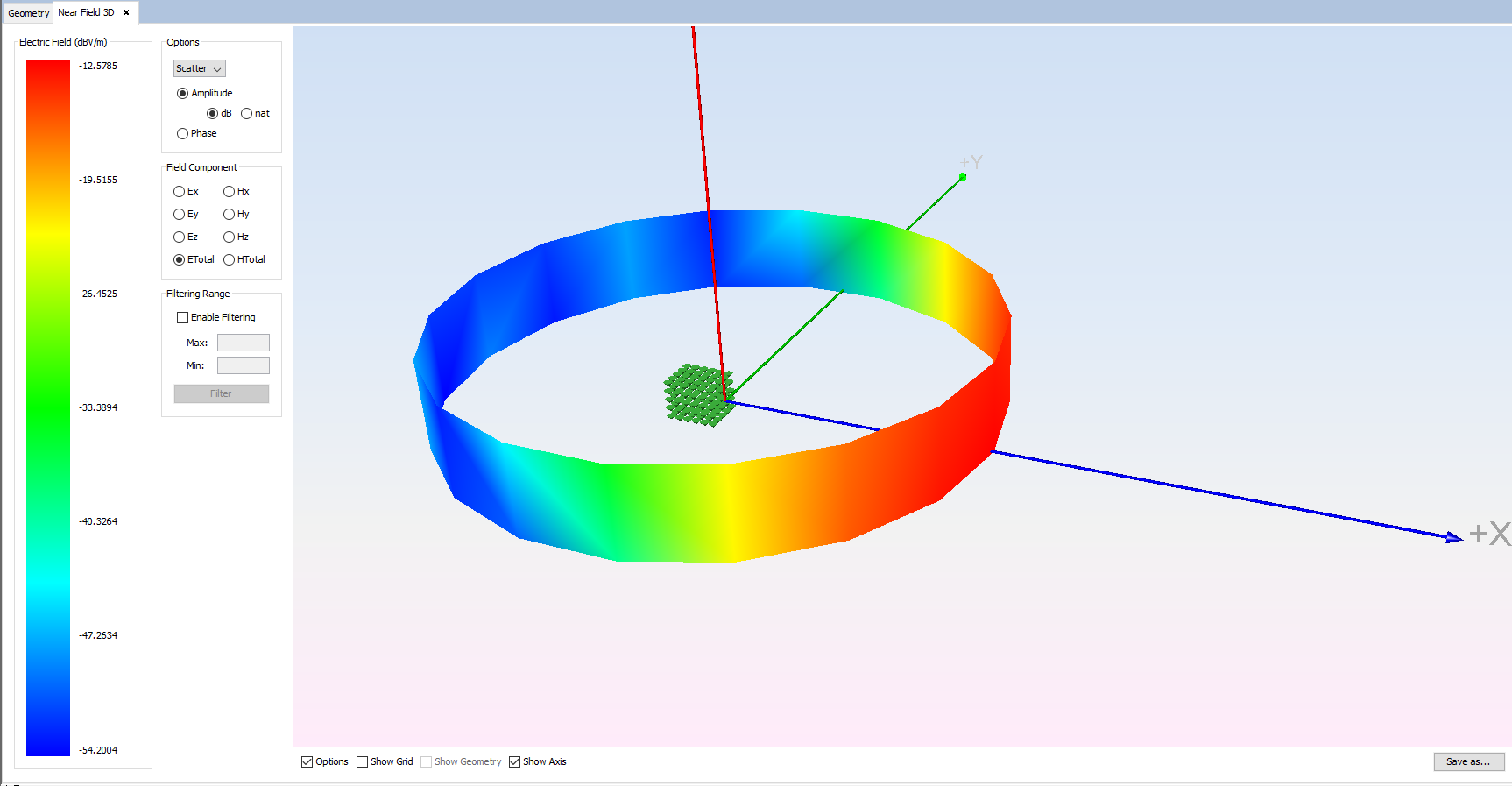
Step 3: Show Results.
Select 'Show Results --> Near Field --> View Near Field Diagram' option to show the observation points diagram. Previously, select the observation to visualize and the step and frequency on the next figure.