Tutorial: Working with Model Hierarchy and Parameterization
Learn how to add a PID controller and dynamics to a water tank model. Learn how to
parameterize the model with context variables and mask super blocks to hide details of the
model hierarchy.
Files for This Tutorial
Watertank.scm
A finished version of the models you build in the tutorials along with any files
required to complete the tutorials are available at this location:
<installation_directory>/tutorial_models/.
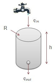
Overview of a Watertank Problem
In a water tank model, a PID controller is added to regulate the flow of water into the
tank.
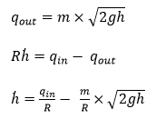
The following flow equations represent the water tank model:
By controlling the inflow rate qin of water into the tank, the water level
h can be reached within a given time. The given system model has only one
input and one output, qin and qout, and therefore requires the addition
of a classic PID controller to control the flow rate of water.
The PID controller is implemented as a super block that is comprised of basic arithmetic and
integration blocks. The coefficients of the Proportional, Integral and Derivative terms of the
PID controller are defined as context variables, which you can edit with OML commands.
The controller in the super block is masked and looks like a regular Activate block. Though the mask hides the implementation details of the super
block, the PID parameters are accessible by double-clicking the super block.
Constructing a PID Controller
Create a model with a PID controller to regulate water flow.
From the ribbon, in the the Files tool group, click .
Save the new model as watertank_practice.scm.
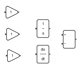
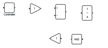
From the Palette Browser, add the following blocks into
your diagram:
From Activate > MathOperations > Gain, drag and drop 3 Gain blocks.
From Activate > Dynamical, drag and drop 1 Integral
block.
From Activate > Dynamical, drag and drop 1 Derivative
block.
From Activate > MathOperations, drag and drop 1 Sum block.
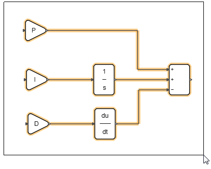
Position the blocks as you see in the following figure:
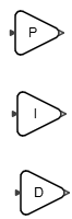
For each Gain block, double-click, enter a value for the Gain parameter, and
then click OK.
For the upper Gain block, enter P.
For the middle Gain block, enter I.
For the lower Gain block , enter D.
Note: Assigning a value P, I, or
D to a parameter indicates that the value
represents a context variable that you will define later in the
tutorial.
Your blocks should look something like this:
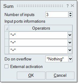
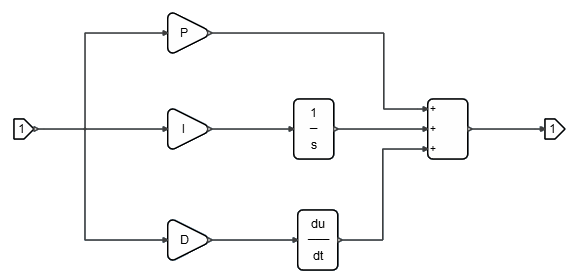
Double-click the Sum block. For Number of inputs, enter
3. In the Signs table, assign
“+” to all inputs:
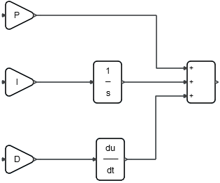
Connect the blocks and adjust the links as you see in the following
figure:
Click and drag your cursor to box-select all of the blocks:
From the ribbon, select the tool, Create Super Block.
The blocks in the diagram convert into a super block:
Double-click the SuperBlock, and the diagram
opens.
From the Palette Browser > Activate > Ports, drag and drop one Input block and one
Output block into the diagram.
Connect the blocks as you see in the following figure:
The Input and Output blocks serve as the interface to exchange signals
from within the super block to the blocks outside of the super
block.
To view the top diagram, in an empty area of the modeling window,
double-click.
The input and output ports should be attached to the super block:
To name the super block, select it, press F2, then enter
Controller.
The name of the super block changes to Controller:
Modeling the Water Tank Dynamics
Construct the dynamics of a water tank based on three flow equations.
From the Palette Browser, add the following blocks to your
diagram:
From Activate > MathOperations, drag and drop two Gain
blocks.
From Activate > MathOperations, drag and drop one Sum block.
From Activate > MathOperations, drag and drop one MathFunc
block.
From Activate > Dynamical, drag and drop one Integral
block.
After adding the blocks, select the MathFunc block,
right-click, and select Flip. Do the same for one of the
Gain blocks.
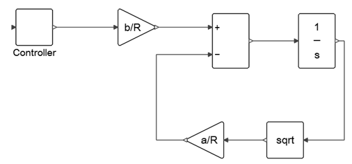
Arrange the blocks as you see in the following figure:
For the upper and lower Gain blocks, double-click, enter a value for the
parameter, Gain, and then click OK.
For the upper Gain block, enter b/R.
For the lower Gain block, enter a/R.
On the MathFunc block, double-click. For the Function
parameter, enter “sqrt”, and then click
OK.
Connect the blocks:
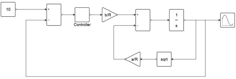
From the Palette Browser, add the following blocks into
your diagram:
From Activate > MathOperations, drag and drop one Sum block.
From Activate > SignalGenerators, drag and drop one Constant
block.
From Activate > SignalViewers, drag and drop one Scope
block.
On the Constant block, double-click. For the parameter,
Constant, enter 10, and then
click OK.
Arrange and connect the blocks:
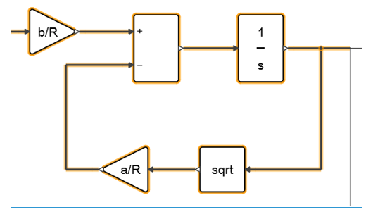
On the diagram, click and drag to box-select the blocks you see in the
following figure:
Right-click and select Super Block.
In the diagram, the blocks in the selected area convert into a super
block. The Super Block operation automatically links the new super block to the
existing blocks in the diagram.
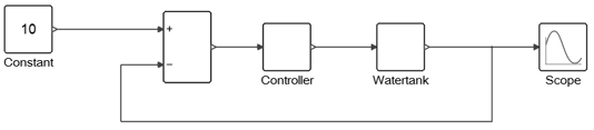
In the Property Editor, select the new super block. Double-click the name field
and enter the name, Watertank.
Modify the connections of the Watertank block to the other blocks in the
diagram:
Save your model.
Defining Context Variables
On the Context tab of the Diagram dialog, enter values for the main and local context
variables.
In an empty area of the root diagram, right-click, and then select
Context, or from the menubar, select the
Diagram tool .
The Diagram dialog opens.
In the Context tab, enter the OML commands as you
see in the following figure, and then click OK.
While the context variables P, I and D are defined in the context of the
main diagram, the variables used elsewhere in the model also receive these
values unless the values are defined in a local context.
On the Watertank super block, double-click.
In an empty area of the main diagram, right-click, and then select
Context.
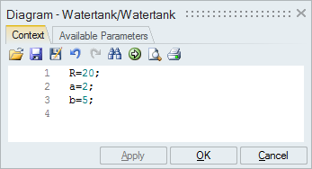
On the Context tab, enter the OML commands as you
see in the following figure, and then click OK.
The context variables R, a and
b are defined in the diagram inside of the super block.
The scope of these variables is semi-global, meaning they are visible only in
the current diagram and any super block in the current diagram. Since the Gain
blocks are in the current diagram and contain the variables
R, a and b, the
variables are defined based on the values specified on the Context tab.
From the ribbon, select Run.
The simulation starts.
In the main diagram, on the Scope block,
double-click.
A Scope window appears.
To fit the view of the Scope in the window, middle-mouse click.
The curve shows the water tank reaches and remains at 10, the designated
level.
Masking the Super Block
Mask the Controller super block and tune the P,
I, and D parameters.
Though the details of the Controller super block are hidden when masked, the
process of editing parameters in a block parameter dialog is the same as for a regular
block.
In the root diagram, select the Controller super block.
From the ribbon, select the Auto Mask tool .
The super block is masked automatically.
On the masked super block, Controller,
double-click.
A parameter dialog appears. As input entries, the parameter values
I, D, and P are
context variables defined in the context of the root diagram.
Select the super block, Controller, and then from the
ribbon, select the Edit Mask
tool.
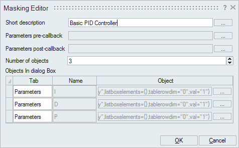
In the Masking Editor dialog, in the Short Description field, enter
Basic PID Controller.
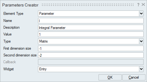
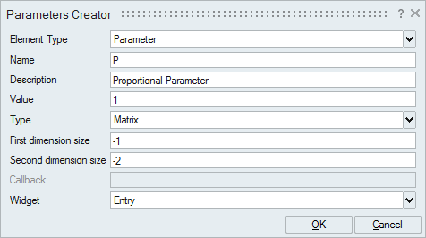
For each parameter, click . In the Parameters Creator dialog, enter the
information as you see in the following figures and click OK.
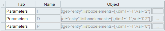
After entering the parameter information, your table should populate like
this:
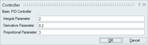
On the Controller super block, double-click. The
parameter descriptions should be updated. Enter numeric values for the
parameters as you see in the following figure:
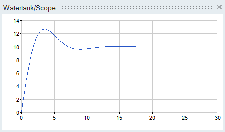
From the ribbon, select Run .
The simulation starts. A Scope window appears with a plot of the
following results:
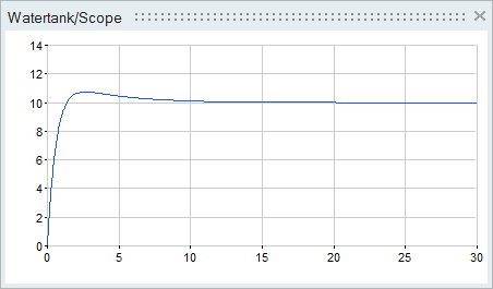
On the super block, Controller, double-click. In the
Proportional Parameter field, enter 8.
Run the simulation again. Your plot should look something like this:
The Scope window shows that the output increases more rapidly at the
beginning, while overshoot is reduced.
 .
.
 .
The blocks in the diagram convert into a super block:
.
The blocks in the diagram convert into a super block:

 .
The Diagram dialog opens.
.
The Diagram dialog opens.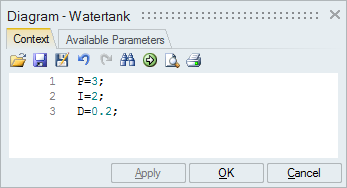

 .
The super block is masked automatically.
.
The super block is masked automatically. tool.
tool.
 . In the Parameters Creator dialog, enter the
information as you see in the following figures and click OK.
. In the Parameters Creator dialog, enter the
information as you see in the following figures and click OK.

 .
The simulation starts. A Scope window appears with a plot of the following results:
.
The simulation starts. A Scope window appears with a plot of the following results: