In this tutorial, you will:
| • | Understand the data in the .out file through analysis |
| • | Load the h3d file from the analysis in HyperView |
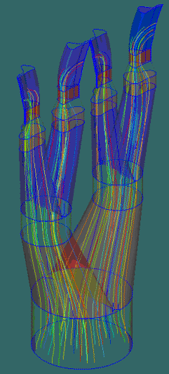
| • | Plot a velocity contour with section cuts to observe the flow pattern in the die |
| • | Plot streamlines to visualize the flow |
| • | Look a heat transfer results |
The goal of post-processing is to understand the behavior of the material flow and heat transfer in the model. In addition, you will also make sure that the results are consistent and the model (mesh and process data) did not introduce any other errors.
The model files for this tutorial are located in the file mfs-1.zip in the subdirectory \hx\MetalExtrusion\HX_1501. See Accessing Model Files.
To work on this tutorial, it is recommended that you copy this folder to your local hard drive where you store your HyperXtrude data, for example, “C:\Users\HyperXtrude\” on a Windows machine. This will enable you to edit and modify these files without affecting the original data. In addition, it is best to keep the data on a local disk attached to the machine to improve the I/O performance of the software.
|
| 1. | Run the solver. The solution convergence history is saved in the file jobname_000.out. |
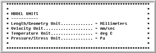
| 2. | Open the file HX_1501_000.out in a text editor. You can verify much of the input data, such as model units, in this file. |
| 3. | Check if the Extrusion Ratio is correct; otherwise, inspect the inflow and outflow boundaries in the model. |
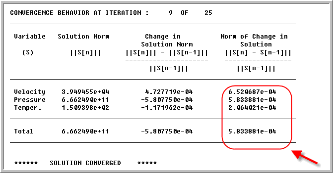
| 4. | Check the Norm on Change in Solution to see whether it is decreasing for velocity, temperature, and pressure as the nonlinear iteration progress. |
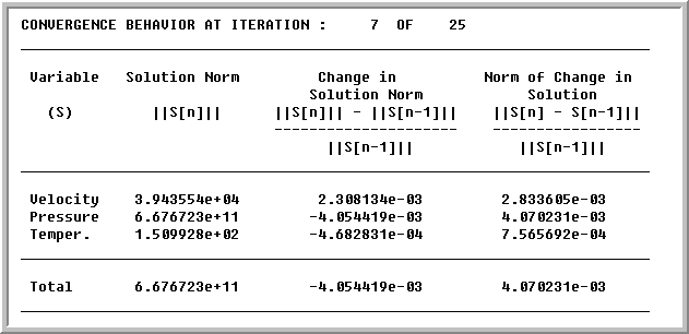
These norms may oscillate initially, but will decrease steadily after a few initial iterations. The solution is converged if the value of Norm of Change in Solution is less than 0.001. HyperXtrude will consider the solution as converged only after all the entries in the last column are less than the tolerance. A slow convergence rate or oscillatory behavior indicates the mesh is too coarse. Fix the problem before proceeding to the next step.
|
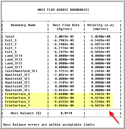
| 1. | Check if the Mass Balance is less than 1 percent. This essentially accounts for law of conservation of mass. In this example, the value is 0.01 percent and it indicates the mass is conserved accurately. |
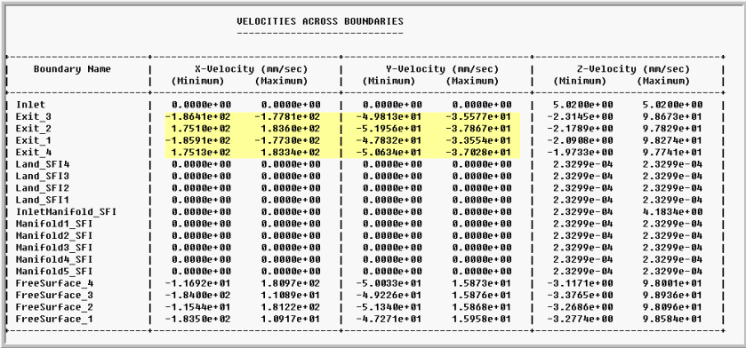
| 2. | Velocity on solid walls must be close to zero. |
| 3. | Velocity on symmetry planes must be equal to zero. |
| 4. | Velocity on free surface boundaries must be small (at least less than four orders of magnitude less than extrusion speed). In this model, it is higher than the acceptable limit. This is because the flow is not balanced for the given die and process conditions. Hence, you will see a significant profile deformation. |
| 5. | The Mass Flux table shows mass flow rate across each boundary. A positive sign indicates material entering through the boundary, and a negative sign indicates material leaving the boundary. The table also contains average velocity of the material entering/leaving through each boundary surface. |
| 6. | If any of these checks fail, verify the boundary conditions. |
|
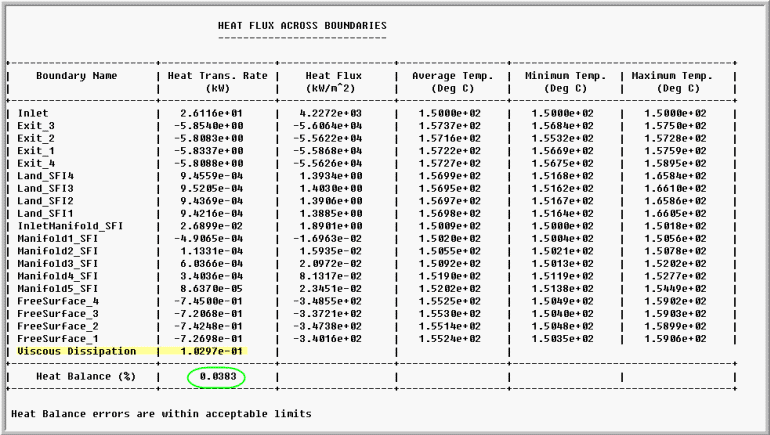
The Heat Flux table shows heat transfer rates across each boundary. A positive sign indicates energy input to the system, and a negative sign indicates energy leaving through the boundary. The table also contains average temperatures at each boundary surface.
| 1. | Check if energy balance is <5 percent. In this model, this is very small - 0.04 percent and indicates a very good energy balance. |
| 2. | Check if average temperatures are within acceptable range. Here, since all the walls are insulated, there is small increase in temperature due to viscous dissipation. |
| 3. | Verify the boundary conditions and material properties if either one of these checks fail. |
|
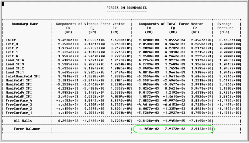
A positive sign indicates force applied on a surface, and a negative sign indicates response. The table also contains average pressure at each boundary surface.
| 1. | Check if each component of total force vector is in equilibrium (<5%). In this model - force balance is very good and the system is in equilibrium. The resultant value is close to 0% in all three components. |
| 2. | Check if average pressure at inlet is within acceptable range. |
| 3. | Verify the boundary conditions and material properties if either on of these checks fail. |
|
The amount of heat generated during deformation must be approximately (within 5%) equal to the mechanical work. This can be computed from the pressure on the inlet face, inlet velocity, area of inlet face, and % work converted to heat. In this model:
| • | Heat Generated - 3.77e+06 x 0.00502 x 0.0062 x 0.9 - 105 W |
| • | Value of viscous dissipation is 103 W (from the Heat Transfer table) |
|
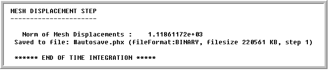
The Norm of Mesh Displacement quantifies the amount of profile deflections. Large values indicate that the velocities at die exit are not uniform and this produces large profile deflections. In this model, the norm is quite high and the die needs corrections.
|
| 1. | Copy the .h3d file HX_1501_000.h3d to your working directory. This file contains the results that can be loaded and reviewed in HyperView. |
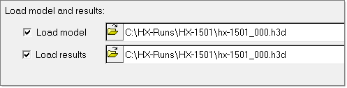
| 2. | Load the .h3d file into HyperView using the Load model option. |
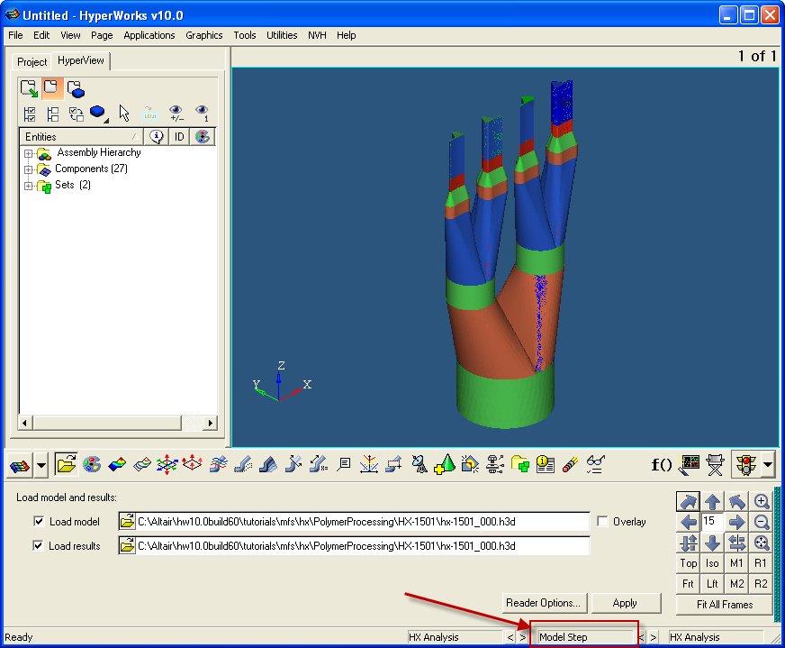
| 3. | Click on the Model Step tab in the bottom pane, and look at the model steps available in the results. The Project pane shows the 2D and 3D sets in the model. The 2D set contains the boundary faces and the 3D set contains the volume mesh. |
|
| 1. | Go to the Contour panel in HyperView. |
| 2. | For Result type:, select Displacement. |
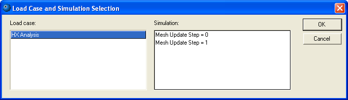
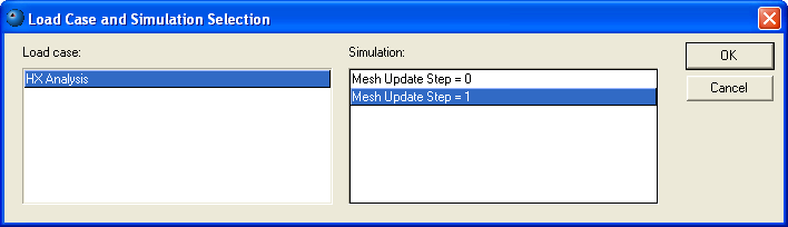
| 3. | Click on the Load case and Simulation selection at the bottom and select Mesh Update Step = 1. |
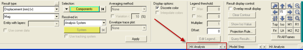
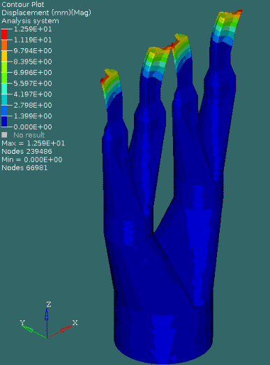
| 4. | Click Apply. The contour shows the displacement of the profile. You will see displacement is significant and it is around 13 mm. |
|
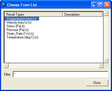
| 1. | In a similar manner, you can inspect other solution components. The list of result types available vary with the model settings. |
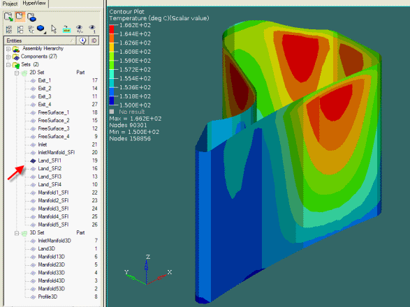
| 2. | You can plot the solution on a boundary surface or a section cut and inspect the data in a variety of ways. In the image below, temperature variation in the land region of exit1 is shown. |
|
| 1. | On the Graphics menu, click Vector  . . |
| 2. | Display only Land3D using the Project Pane. |
| 3. | Set the following data as shown below: |
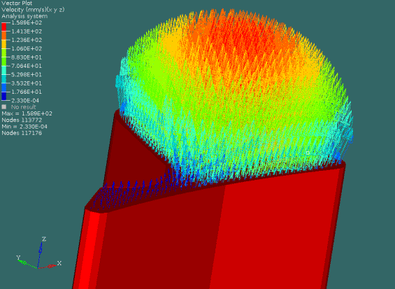
| 4. | Select some nodes using the graphics window, or select all nodes. In the image below, the top layer of nodes in land of exit1 was selected using the graphics window. |
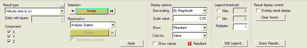
| 5. | Click Apply to display the vectors. |
|
Return to Polymer Processing Tutorials