Example 3

In this example, the Monostatic RCS of two cubes is calculated, where one cube is dynamic.

Step 1

Create a new project following steps 1 to 5 in Example1 above.

Step 2

Click on Geometry → Solid → Box.

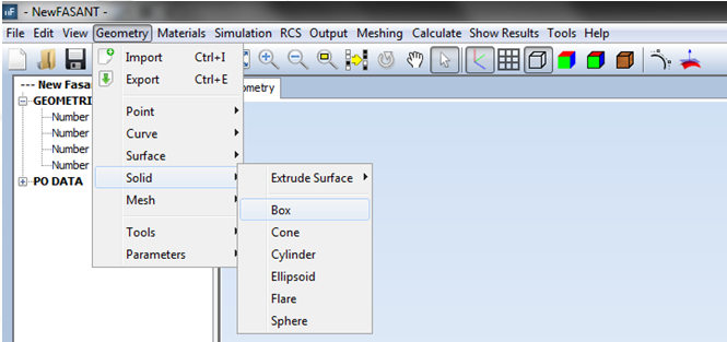
Figure 1. Create box command

Create the first box by entering the following parameters from the command line as shown in the next Figure.

· First corner of base [x y z] 0.5 -0.5 0

· Base size [width depth] 1 1

· Height 1

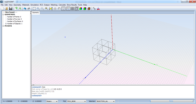
Figure 2. Box Parameters box

Step 3

Now, let’s add the dynamic cube to the model. We want this cube to move in the direction of the positive Z-axis at 0.5 meters each step in the simulation. We will use three steps for this simulation.

First, we must define a parameter for the geometry that represents the Z coordinate of the base of the cube at each step of the simulation. To do this, select Geometry → Parameters → Define Parameters and the following window appears:

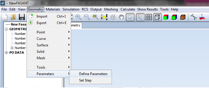
Figure 3. Define parameters

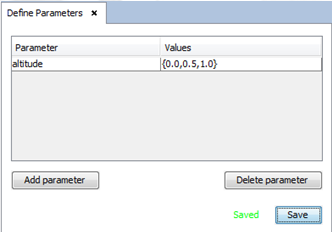
Figure 4. Define parameters panel

Press the Add parameter button, after which a row appears in the table. In the Parameter column, change the name of the created parameter to “height”, for example. Then change the values to “{0.0, 0.5, 1.0}” and left-click the Save button to save the changes.

Now, create a new box as the other. It is possible to change the parameters as desired, but the z coordinate of the first corner of the base must be now the parameter “altitude”.

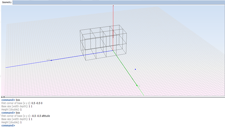
Figure 5. Creating the dynamic cube

Optional: To see a visualization of each step for the second cube, select the Geometry → Parameters → Set Step. Enable “Linear (By step)”, set the desired time delay between steps, and left-click Run to see the animation on the Geometry View.

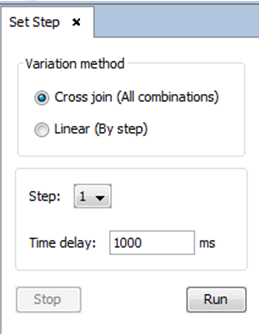
Figure 6. Execute Parameters box

It is possible to see the two remaining steps for the simulation in the next Figures.

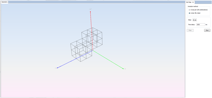
Figure 7. View of the dynamic cube (Step 2)

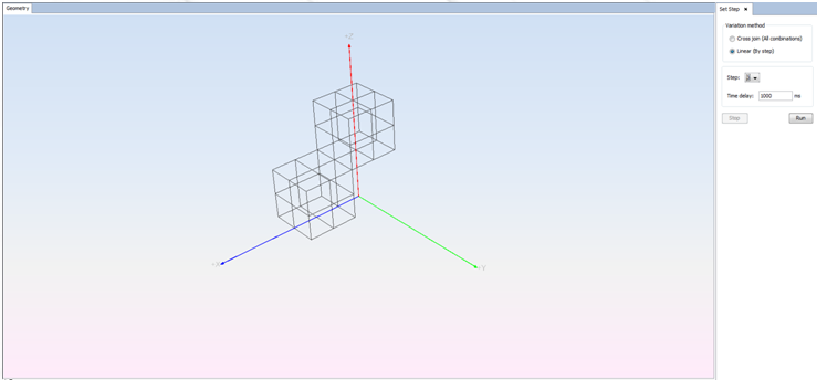
Figure 8. View of the dynamic cube (Step 3)

Step 4: Click on Simulation → Parameters. Enter the simulation parameters as shown in the next Figure.

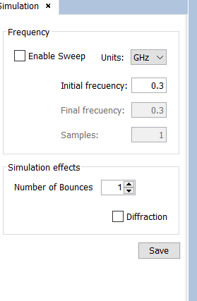
Figure 9. Simulation parameters

Step 5

Select RCS → Parameters and enter the parameters shown in the next Figure.

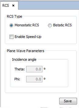
Figure 10. RCS parameters

Step 6

Select Output → Observation Directions and enter the parameters shown in the next Figure.

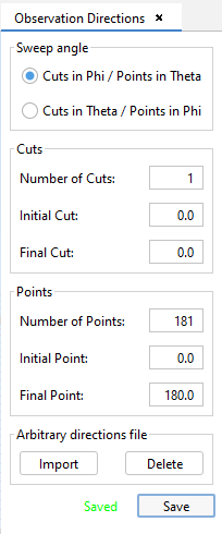
Figure 11. Observation Directions panel

Step 7

Select Meshing → Create Mesh. Select the appropriate number of processors available to run the meshing process as shown in the next Figure and left-click Mesh.

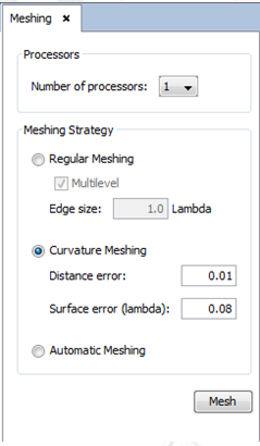
Figure 12. Meshing configuration

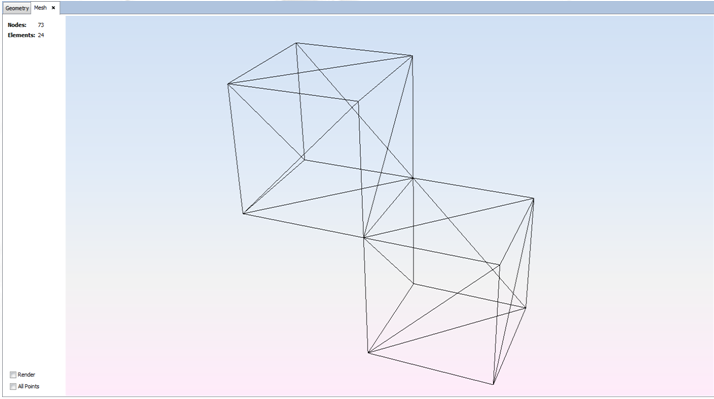
Figure 13. Resulting Mesh

Step 8

Select Calculate → Execute and enter the number of available processors for this simulation.

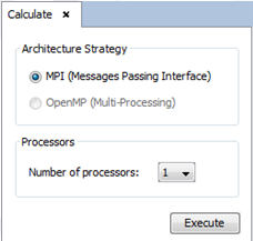
Figure 14. Calculate options

Step 9

Click on Show Results → Far Field → View Cuts, to show the RCS graph.

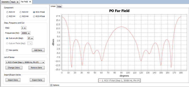
Figure 15. RCS graphic of the first step

The plot corresponds to the RCS of the first step (when the two boxes share the same Z coordinate). To plot the graphics for the remaining two steps, select “2” in the Step combo-box and left-click the Add Series button. Repeat this procedure to add Step 3 to the RCS graphic.

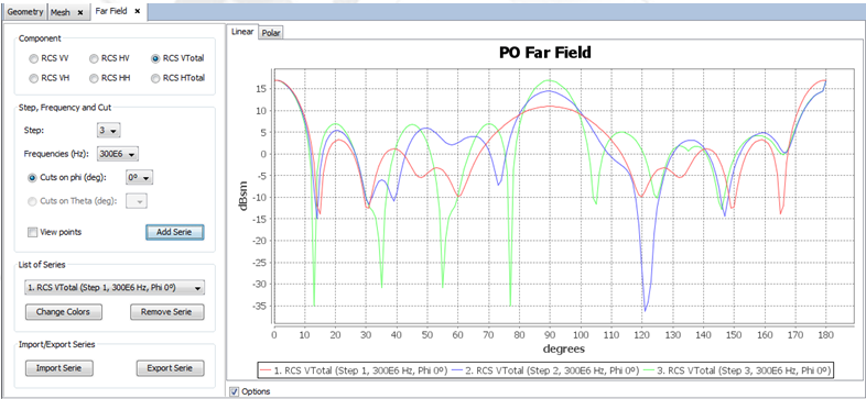
Figure 16. RCS graphic showing each step

Step 10

Click on Show Results → Far Field → View Text Files, to show the RCS data file. Select the step to obtain as a data file. Press OK to continue.

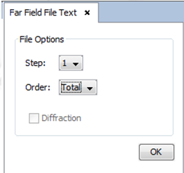
Figure 17. View Text Files options

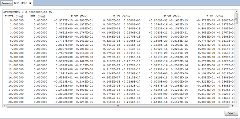
Figure 18. Far-Field text file