Damping Models
Constant Damping Model
The linear damping force is computed according to the law:
- ci
- Constant damping value, and is found in the [CONSTANT_DAMPING_xx] block for the ith force direction in the property file.
- v
- Deformation velocity in the bushing in the ith force direction.
Rubber Damping Model
Schematics and Equation
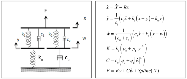
Figure 1.
- X
- The input displacement provided to the bushing
- y and w
- The internal states of the bushing
- k0 and k1
- Represent the bushing rubber stiffness
- k2
- Used to control the stiffness at large velocities
- c0
- Produces the roll-off observed in the experimental data at low velocities
- c1
- Accounts for the relaxation of the bushing impact force
- c2
- Represents the viscous damping observed at large velocities
- R
- The cutoff frequency associated with a first order filter that acts on the input X
- x
- The dynamic content of the bushing input X. This is the filter output.
- and
- The time derivatives of the internal states of the bushing y and w
- K
- The effective stiffness of the bushing
- C
- The effective damping of the bushing
- Spline (X)
- The static force response of the bushing.
- The effective stiffness K is
k0 multiplied by a
factor:
(2) - Similarly, the effective damping C is
c0 multiplied by a
factor:
(3)
- Static force at the operating point: Spline (X)
- Force due to the dynamic behavior of the bushing:
First Order Filter
A first order filter, with cutoff frequency R, is used to identify the dynamic component, x, of the input signal, X. The transfer functions of the signal sent to the dynamic and the static models, assuming X0=0, are:
TF of signal to dynamic model=
TF of signal to dynamic model=1
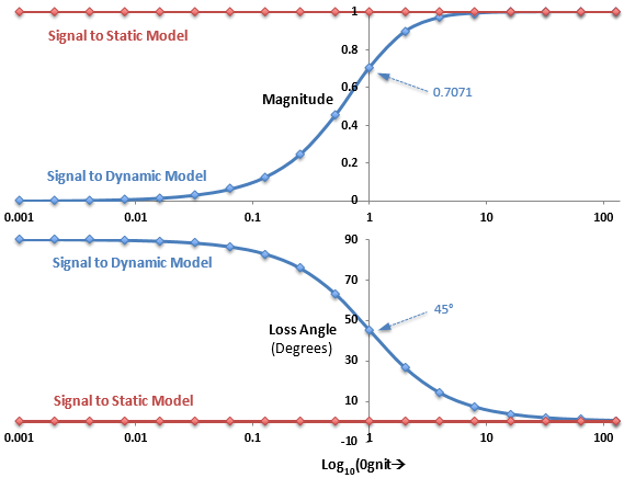
Figure 2.
- The top figure plots the magnitude of the transfer function against Log10(ω/R).
- The bottom figure plots the loss angle of the transfer function against Log10(ω/R).
- Plots of the signal sent to the dynamic model are gray-blue.
- Plots of the signal sent to the static model are brick-red.
- When (ω/R) << 1, that is at low frequencies, then:
- The magnitude of the signal sent to the dynamic model is close to 0.
- The loss angle of the signal sent to the dynamic model is close to 90°.
- The magnitude of the signal sent to the static model is 1.
- The loss angle of the signal sent to the static model is 0°.
The bushing essentially behaves as the static model. The loss angle of the signal sent to the dynamic model is close to 90°, but this is not important since the magnitude of the signal is close to zero.
- When (ω/R) >> 1, that is at high frequencies, then:
- The magnitude of the signal sent to the dynamic model is close to 1.
- The loss angle of the signal sent to the dynamic model is close to 0° .
- The magnitude of the signal sent to the static model is 1.
- The loss angle of the signal sent to the static model is 0°.
The bushing essentially behaves as a dynamic model superimposed on top of a static model.
- When (ω/R) = 1, that is at the cut-off frequency, then:
- The magnitude of the signal sent to the dynamic model is
- The loss angle of the signal sent to the dynamic model is 45°.
- The magnitude of the signal sent to the static model is 1.
- The loss angle of the signal sent to the static model is 0°.
The bushing essentially behaves as a dynamic model superimposed on top of a static model.
Scale Factors P0, P1, P2 and Q0, Q1, Q2
These factors are used to represent friction in the bushing material and also other effects such as viscoelasticity.
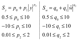
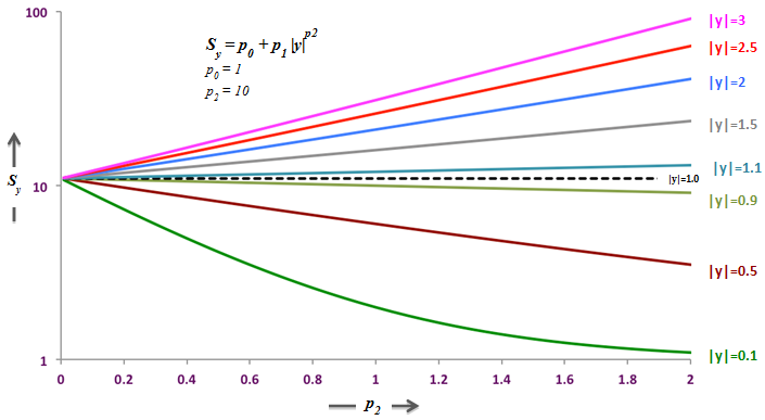
Figure 3.
The functional form of Sy is selected as it easily represents a variety of shapes with very few parameters. Note that Sy and Sw are primarily responsible for capturing the dependency of the dynamic stiffness and loss angle on the amplitude of the input.
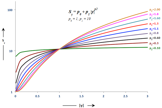
Figure 4.
Multiple Preloads
The following equations show the method for computing the bushing output for multiple preloads.
- n be the number of preloads in the test data; i be the current load case.
- Pi be the preload corresponding to the ith load case.
- Sort the preloads Pi and renumber the preloads such that P1 < P2 < … < Pn.
- xi be the filter output corresponding to the ith load case.
- F0i be the static response of the bushing corresponding to the ith load case.
- fi be the dynamic response corresponding to the ith load case.
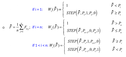
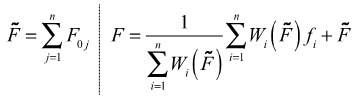
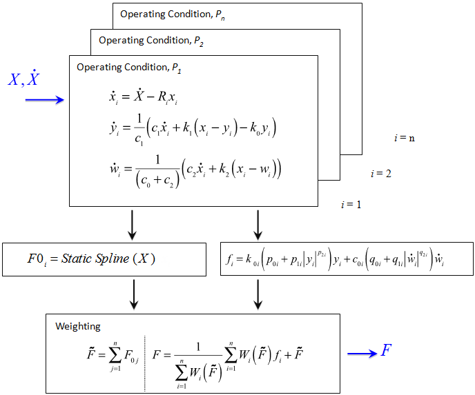
Figure 5.
Factor RMIN
During simulation, an additional parameter RMIN is provided for you. If the fitted value of R is greater that RMIN, then the fitted value is used, otherwise RMIN is used. During run time, R affects how quickly the bushing responds to changes in the input.
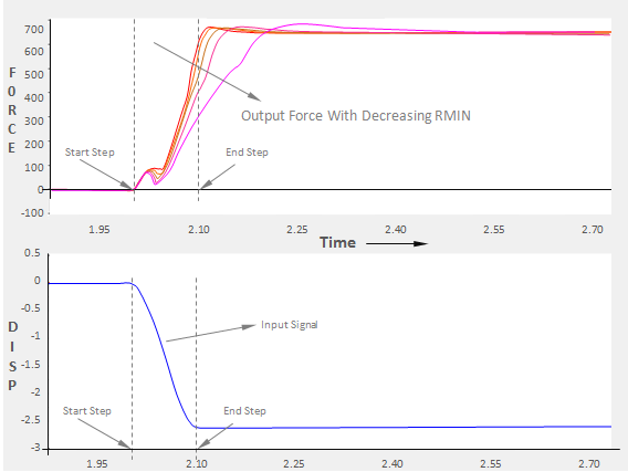
Figure 6.
A large value of R implies that most of the signal is classified as steady state, so the static effects, which react instantaneously to input changes, will dominate. In contrast, when R is small, most of the signal is classified as transient. Therefore bushing internal dynamics will dominate the response and the response will be somewhat slower.
Lower Bound of R and RMIN Selection
The choice of a lower bound of R is essential to achieve a result that shows the correct characteristics for low frequencies and preload dependent simulations.
The lower bound you chose for R during fitting depends on how the bushing is going to be used during simulation and on the available test data. If the application isn’t known at the time of fitting, the lower bound may be chosen only according to the test data. In a concrete application that value of R can then be modified in the simulation model by setting RMIN accordingly.
Choosing the Lower Bound of R from the Test Data
The desired behavior for a bushing model is that input frequencies that are smaller than the lowest provided test frequency data f0 be passed into the static spline. To achieve this behavior, the lower limit of R should be set greater or equal to 2f0.
Choosing the Lower Bound of R Based on Anticipated Usage During Simulation
If you desire that the simulation model have the ability to switch between two preloads within a given time , then you should choose R to be greater or equal to
If you decide that these values of R are too conservative or you don’t want the entire response from the static spline, the simulation model is still capable of doing the switch between these preloads. The time it takes to complete a switch of all states from one preload to another is given by .
Hydromount Damping Model
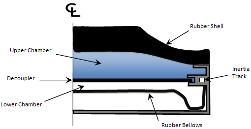
Figure 7.
At low displacement amplitudes, fluid in the upper chamber simply deflects the decoupler. The hydromount behaves just like a rubber bushing. As the input displacement increases, the fluid in the upper chamber flows into the lower chamber. With increasing displacement, fluid effects start to dominate and the behavior of the hydromount changes dramatically.
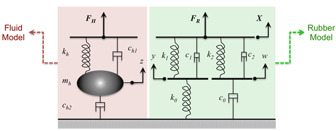
Figure 8.
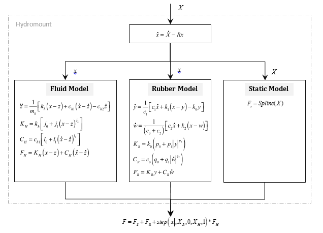
Figure 9.
Inputs
- X is the input displacement provided to the bushing.
- R is the cutoff frequency associated with a first order filter.
- The filter removes the steady state deformation of the bushing and passes only the transient portion of the input, x, to the dynamic models. The full input, X, is channeled to the static model.
Outputs
- The force due to the fluid behavior, FH, which is turned on gradually.
- The force due to deformation in the rubber component, FR.
- The static force at the operating point, which is computed from the static spline that is provided.
XR is a design parameter that defines the deformation at which the fluid force transition begins.
XH is a design parameter that defines the deformation at which the fluid force transition ends.
Quite often, the test data for a hydromount does not capture the transition from pure rubber to full hydromount behavior. XR and XH are therefore not fitted, and are available for you to modify in the .gbs. The default values of XR and XH are such that the STEP function always returns 1.0.
- z is an internal state representing fluid motion.
- mh represents the equivalent fluid mass.
- kh is the coupling stiffness between rubber and fluid.
- ch1 is the coupling damping between rubber and fluid.
- ch2 is the fluid damping.
- jo, j1, j2 and l0, l1, l2 model the amplitude dependence in the fluid equations.
- KH is the effective fluid stiffness in the bushing.
- CH is the effective fluid damping in the bushing.
- y and w are the internal states of the bushing.
- k0 and k1 represent the bushing stiffness.
- k2 is used to control the stiffness at large velocities.
- c0 produces the roll-off observed in the experimental data at low velocities.
- c1 produces the roll-off observed in the experimental data at low velocities.
- c2 represents the viscous damping observed at large velocities.
- po, p1, 2 and qo, q1, q2 model the amplitude dependence in the rubber equations.
- K is the effective stiffness of the bushing.
- C is the effective damping of the bushing.
- Spline (X) is the static force response of the bushing.
Filter implementation, multiple preload support, and the use of RMIN are exactly the same as for the rubber bushing.