ACU-T: 6106 AcuSolve - EDEM Bidirectional Coupling with Mass Transfer
Prerequisites
This tutorial introduces you to the workflow for setting up and running a basic AcuSolve-EDEM bidirectional coupling simulation with mass transfer. Prior to starting this tutorial, you should have already run through the introductory HyperWorks tutorial, ACU-T: 1000 HyperWorks UI Introduction and ACU-T: 6100 Particle Separation in a Windshifter using Altair EDEM, and have a basic understanding of HyperWorks CFD, AcuSolve, and EDEM. To run this simulation, you will need access to a licensed version of HyperWorks CFD, AcuSolve, and EDEM.
Prior to running through this tutorial, copy HyperWorksCFD_tutorial_inputs.zip from <Altair_installation_directory>\hwcfdsolvers\acusolve\win64\model_files\tutorials\AcuSolve to a local directory. Extract the files from the folder named ACU6106_EDEM_MassTransfer located in HyperWorksCFD_tutorial_inputs.zip.
Problem Description
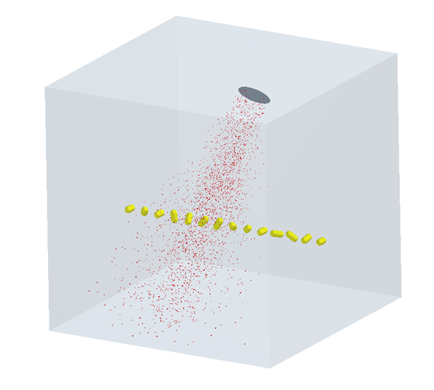
Figure 1.
By activating heat transfer and coupling with AcuSolve, this API can also be used to simulate the drying process of tablets. Using coupled heat and mass transfer, the amount of coating that has evaporated can be tracked. In this tutorial, a simple tablet coating and drying process is simulated where spray particles are injected from t=0 to t=0.25 seconds. As the spray particles interact with the tablet particles, the particles in the center receive a certain amount of coating. The spray injection is stopped at t=0.25s and the tablets are allowed to dry for the next 0.25 seconds. As the time progresses, you will observe that the coating evaporates gradually and the ‘AddedVolume’ decreases.
Part 1 - EDEM Simulation
Start Altair EDEM from the Windows start menu by clicking .
Open the EDEM Input Deck
-
In the dialog, browse to your problem directory and open the
tablet.dem file.
The geometry and the materials are loaded.
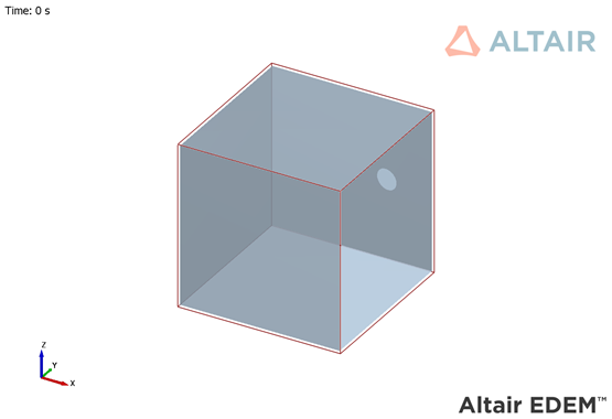
Figure 2.
Review the Bulk Material and Particle Shape
-
Under Bulk Material, click spray and verify that the
properties are set as shown below.
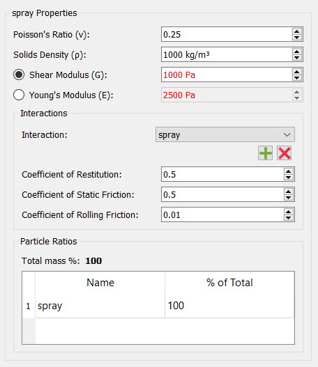
Figure 3. -
Click the tablet bulk material and verify that the
properties are set as shown below.
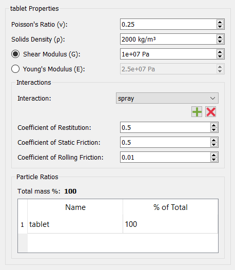
Figure 4. -
Click Properties under tablet and review the tablet
shape.
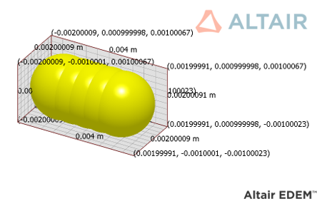
Figure 5.
Set the Physics Models
-
Set the Interaction to Particle to Particle then click
Edit Contact Chain.
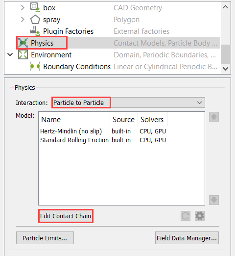
Figure 6. -
In the dialog, activate the checkbox for the
spray_example plug-in model. Set the Base and
Friction models as shown in the figure below and click
OK.
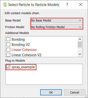
Figure 7.Note: If you do not see the spray_example plug-in model, please make sure that you place the spray_example.dll (for Windows) and spray_example.so (for Linux) files in the problem directory. -
In the dialog, activate the checkboxes for Temperature
Update and spray_example then click
OK.
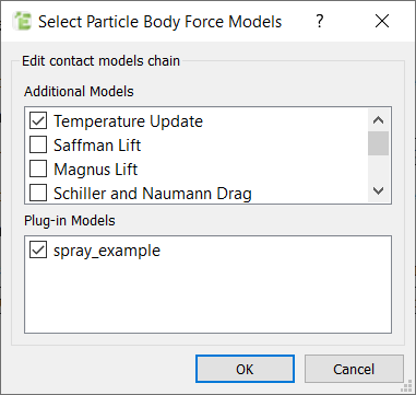
Figure 8. -
In the Creator Tree, select Temperature Update then
click
 .
.
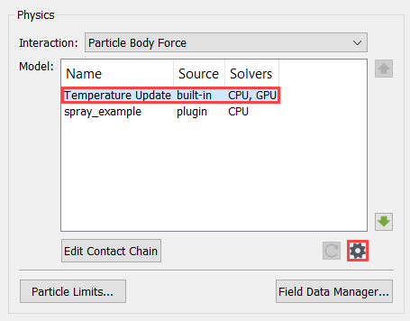
Figure 9.
Define Geometries and Factories
-
Verify that the Factory Type is set to static and set
the particle generation parameters as shown in the figure below. Make sure that
the Material/Meta-Particle is set to tablet.
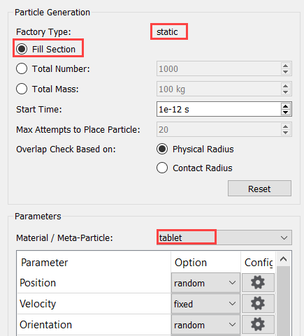
Figure 10. -
Under Parameters, set the Position option to cubic then
click .
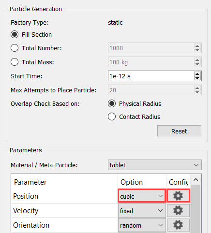
Figure 11. -
In the dialog, enter the position parameters as shown in the figure below then
click OK.
This creates a row of tablet particles spaced evenly along the y-axis and located at the center of the box.
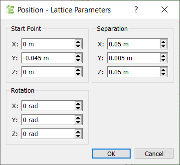
Figure 12. -
Similarly, click next to the Temperature setting,
set the particle temperature to 350 K, then click
OK.
-
Set the particle generation parameters as shown in the figure below. Set the
Material to spray.
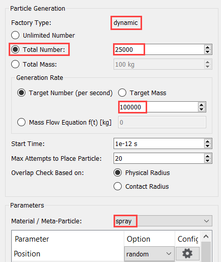
Figure 13. -
Under Parameters, set the Velocity option to spray then
click .
-
In the dialog, set the spray velocity parameters as shown in the figure below
then click OK.
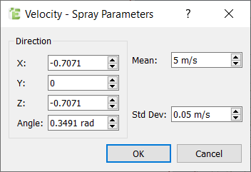
Figure 14. -
Similarly, click next to the Temperature setting,
set the particle temperature to 350 K, then click
OK.
Define the Simulation Settings
-
Click
 in the top-left corner to go to
the EDEM Simulator tab.
in the top-left corner to go to
the EDEM Simulator tab.
-
Set the Selected Engine to CPU Solver and set the Number
of CPU Cores based on availability.
Figure 15.
Part 2 - AcuSolve Simulation
Start HyperWorks CFD and Open the HyperMesh Database
-
From the Home tools, Files tool group, click the Open Model tool.

Figure 16.The Open File dialog opens.
Validate the Geometry
The Validate tool scans through the entire model, performs checks on the surfaces and solids, and flags any defects in the geometry, such as free edges, closed shells, intersections, duplicates, and slivers.
Figure 17.
Set Up Flow
Set the General Simulation Parameters
-
From the Flow ribbon, click the Physics tool.

Figure 18.The Setup dialog opens. -
Set the Number of passive species to 1.
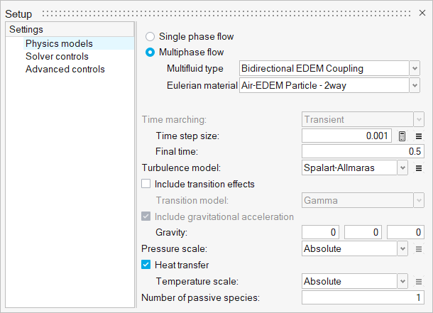
Figure 19. -
Click the Solver controls setting. Set the Minimum and
Maximum stagger iterations to 0 and
2, respectively.
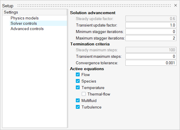
Figure 20.
Assign Material Properties
-
From the Flow ribbon, click the Material tool.

Figure 21. -
On the guide bar, click
 to exit
the tool.
to exit
the tool.
Generate the Mesh
-
From the Mesh ribbon, click the
Volume tool.

Figure 22.The Meshing Operations dialog opens. -
Deactivate Curvature-based surface refinement then click
Mesh.
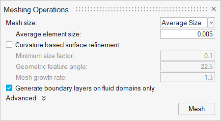
Figure 23.
Define Nodal Outputs
Once the meshing is complete, you are automatically taken to the Solution ribbon.
-
From the Solution ribbon, click the Field tool.

Figure 24.The Field Output dialog opens. -
Set the Time step interval to 0.01.
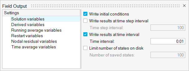
Figure 25.
Submit the Coupled Simulation
-
Start the coupling server by clicking Coupling Server in
EDEM.

Figure 26.Once the Coupling server is activated, the icon changes.
Figure 27. -
From the Solution ribbon, click the Run tool.

Figure 28.The Launch AcuSolve dialog opens. -
Click Run to launch AcuSolve.
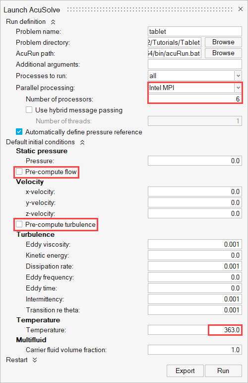
Figure 29.Once the AcuSolve run is launched, the Run Status dialog opens. -
In the dialog, right-click on the AcuSolve run and
select View log file.
If the coupling with EDEM is successful, that information is printed in the log file.
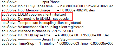
Figure 30.Once the simulation is complete, the summary of the run time is printed at the end of the log file.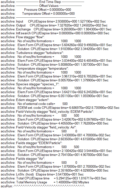
Figure 31.
Post-Process the Results with EDEM
-
Once the EDEM simulation is complete, click
 in the top-left corner to go to
the EDEM Analyst tab.
in the top-left corner to go to
the EDEM Analyst tab.
-
Verify that the Display Mode is set to Filled and set
the Opacity to 0.2.
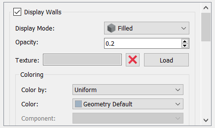
Figure 32. -
Click Apply All.
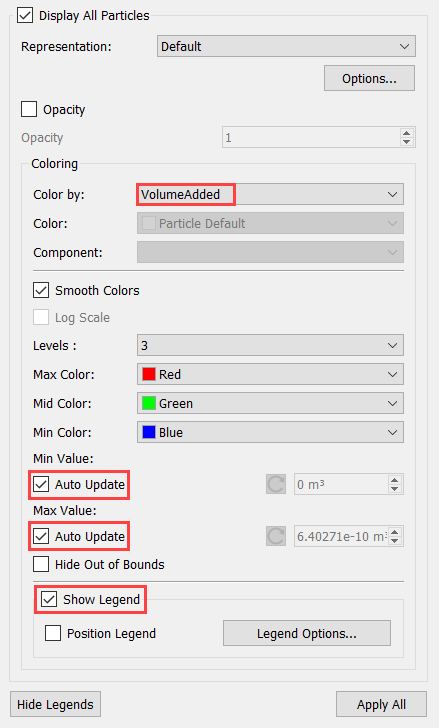
Figure 33. -
On the menu bar, set the time to
0 by clicking:

Figure 34. -
Set the View plane to Default.

Figure 35. -
In the Viewer window, set the Playback Speed to 0.1x and
then click
 to play the particle flow animation.
Figure 36.Observe that the added volume increases in the beginning as the tablets receive the spray coating. Once the spray injection is stopped, the coating starts to dry up and the added volume decreases gradually.
Summary
In this tutorial, you have learned how to set up and run a basic AcuSolve-EDEM bidirectional (two-way) coupling problem with mass transfer. You learned how to create particles with specific position and internal spacing and also learned how to define a spray injection. Once the simulation was completed, you processed the results to view the coating variation over time.