ACU-T: 5200 Rigid-Body Dynamics of a Check Valve
This tutorial provides the instructions for setting up, solving and viewing results for a simulation of the opening of a pressure check valve. In this simulation, AcuSolve is used to compute the forces on the valve due to the time-varying inlet flow field and to compute the motion of the valve that results from these flow forces. This tutorial is designed to introduce you to a number of modeling concepts necessary to perform simulations of rigid-body dynamics.
- Transient simulation
- Use of a multiplier function to scale inlet boundary condition values
- Mesh motion
- Fluid-structure interaction with a rigid body
- Post-processing with AcuProbe
- Results animation
Prerequisites
You should have already run through the introductory tutorial, ACU-T: 2000 Turbulent Flow in a Mixing Elbow. It is assumed that you have some familiarity with AcuConsole, AcuSolve, and AcuFieldView. You will also need access to a licensed version of AcuSolve.
Prior to running through this tutorial, copy AcuConsole_tutorial_inputs.zip from <Altair_installation_directory>\hwcfdsolvers\acusolve\win64\model_files\tutorials\AcuSolve to a local directory. Extract pressureCheckValve.x_t from AcuConsole_tutorial_inputs.zip.
Analyze the Problem
An important first step in any CFD simulation is to examine the engineering problem to be analyzed and determine the settings that need to be provided to AcuSolve. Settings can be based on geometrical components (such as volumes, inlets, outlets, or walls) and on flow conditions (such as fluid properties, velocity, or whether the flow should be modeled as turbulent or as laminar).
The problem to be addressed in this tutorial is shown schematically in Figure 1. It consists of a cylindrical pipe containing water that flows past a check valve with a shutter attached to a virtual spring (not included in the geometry). The inlet pressure varies over time and the movement of the shutter will be determined as a function of the balance of the fluid forces against the reactive force of the spring. The problem is rotationally periodic at 30° increments about the longitudinal axis, and it is assumed that the resulting flow is also rotationally periodic, allowing for modeling with the use of a wedge-shaped section. For this tutorial, a 30° section of the geometry is modeled, as shown in the figure. Modeling a portion of an rotationally periodic geometry leads to reduced computation time while still providing an accurate solution.

Figure 1. Schematic of Check Valve with Spring-Loaded Shutter
The pipe has an inlet diameter of 0.08 m, and is 0.4 m long. The check-valve assembly is 0.085 m downstream of the inlet. It consists of a plate 0.005 m thick with a centered orifice 0.044 m in diameter and a shutter with an initial position 0.005 m from the opening, simulating a nearly closed condition. The shutter plate is 0.05 m in diameter and 0.005 m thick. The shutter plate is attached to a stem 0.03 m long and 0.01 m in diameter. The mass of the shutter and stem is 0.2 kg and its motion is affected by a virtual spring with a stiffness of 2162 N/m. The motion of the valve shutter is limited by a stop mounted on a perforated plate downstream of the shutter.
Note that AcuSolve's internal rigid-body-dynamics solver is not able to simulate contact. Therefore, this problem is formulated to avoid contact between the valve and the stop.
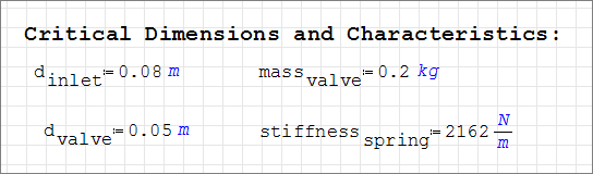
Figure 2.
- Scale up the fluid forces calculated by AcuSolve by a factor
of 12 to represent the full load on the device when the displacement of the body is
computed.
Using this approach, the full stiffness of the valve spring is used in the rigid-body solution, and the full mass of the valve is used.
- Scale down the mass of the valve and the stiffness of the spring to by a factor of 12 to
match the fraction of the valve geometry to be modeled.
Using this approach, the loading passed to the rigid-body solver is not scaled.
This second approach is used in this tutorial; the scaled mass of 0.0167 kg and the scaled stiffness of 180.1667 N/m will be used .
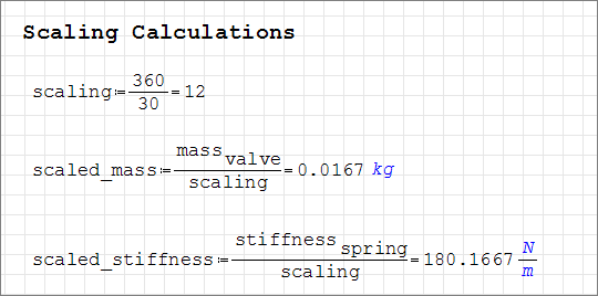
Figure 3.
The fluid in this problem is water, which has a density (ρ) of 1000 kg/m3 and a molecular viscosity (μ) of 1 X 10⁻³ kg/m-sec, as shown in the worksheet.
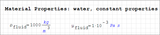
Figure 4.
At the start of the simulation the flow field is stationary. Flow is driven by the pressure at the inlet, which varies over time as a piecewise linear function shown in Figure 5. As the pressure at the inlet rises, the flow will accelerate as the valve opens. The turbulence viscosity ratio is assumed to be 10.
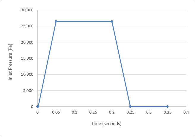
Figure 5. Transient Pressure at the Inlet
Prior simulations of this geometry indicate that the average velocity at the inlet reaches a maximum of 0.9 m/s. At this velocity, the Reynolds number for the flow is 72,000. When the Reynolds number is above 4,000, it is generally accepted that flow should be modeled as turbulent.
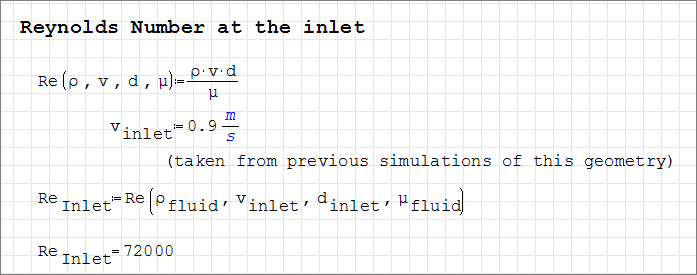
Figure 6.
Note that the initial conditions of the flow are actually laminar, however, the increase in flow velocity and flow around the valve shutter is expected to cause a rapid transition to turbulent conditions. Therefore, the simulation will be set up to model transient, turbulent flow. When performing a transient analysis, convergence is achieved at every time step based on the defined stagger criteria. Mesh motion will be modeled using arbitrary mesh movement (arbitrary Lagrangian-Eulerian mesh motion).
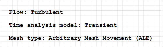
Figure 7.
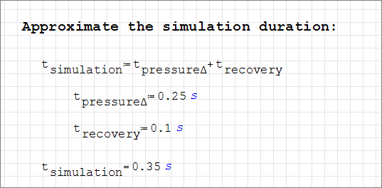
Figure 8.
Another critical decision in a transient simulation is choosing the time increment. The time increment is the change in time during a given time step of the simulation. It is important to choose a time increment that is short enough to capture the changes in flow properties of interest, but does not require unnecessary computation time.
There are two methods commonly used for determining an appropriate time increment. The first method involves identification of the time scales of the transient behaviors of interest and setting the time increment to sufficiently resolve those behaviors. The second method involves setting a limit on the number of mesh elements that the flow can cross in a given time step. A convenient metric for the number of mesh elements crossed per time step is the Courant-Friederichs-Lewy number, or CFL number. With this method, the time increment can be computed from the mesh size, the flow velocity, and the desired CFL number.
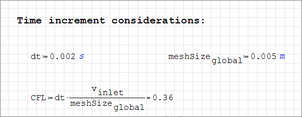
Figure 9.
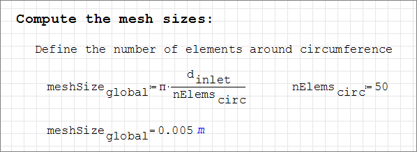
Figure 10.
AcuSolve allows for mesh refinements in a user-defined region that is independent of geometric components of the problem such as volumes, model surfaces, or edges. It is useful to refine the mesh in areas where gradients in pressure, velocity, eddy viscosity, and the like are steep.
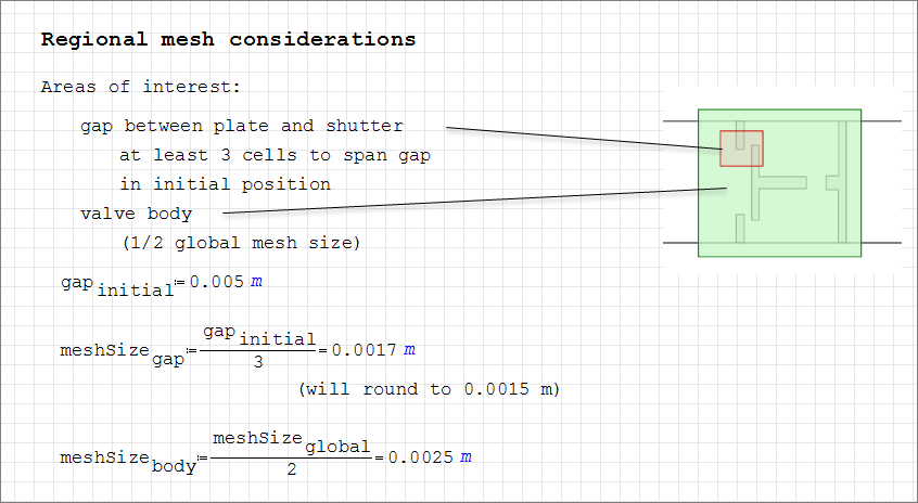
Figure 11.
Once a solution is calculated, the flow properties of interest are the displacement of the moving surface, the mass flow rate at the outlet, pressure contours on the symmetry plane, and velocity vectors on the symmetry plane.
Define the Simulation Parameters
Start AcuConsole and Create the Simulation Database
In this tutorial, you will begin by creating a database, populating the geometry-independent settings, loading the geometry, creating groups, setting group attributes, adding geometry components to groups, creating a multiplier function, and assigning mesh controls and boundary conditions to the groups. Next you will generate a mesh and run AcuSolve to simulate the transient behavior. You will use AcuProbe to post-process mesh displacement and mass flow. Finally, you will visualize the results using AcuFieldView.
In the next steps you will start AcuConsole, create the database for storage of AcuConsole settings, and set the location for saving mesh and solution information for AcuSolve.
Set General Simulation Attributes
In the next steps you will set attributes that apply globally to the simulation. To simplify this task, you will use the BAS filter in the Data Tree Manager. The BAS filter limits the options in the Data Tree to show only the basic settings.
The general attributes that you will set for this tutorial are for turbulent flow, transient time analysis, and the use of arbitrary mesh movement.
-
Click BAS in the Data Tree Manager to switch to basic view in the Data Tree.
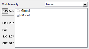
Figure 12. -
Double-click the Global
Data Tree item to expand it.
Tip: You can also expand a tree item by clicking
 next to the item name.
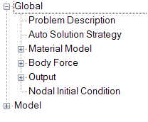
Figure 13. -
Change the Mesh type to Arbitrary Mesh Movement
(ALE).
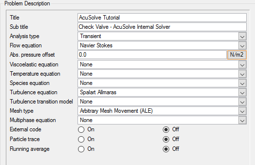
Figure 14.
Set Solution Strategy Attributes
In the next steps you will set attributes that control the behavior of AcuSolve as it progresses during the transient solution.
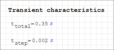
Figure 15.
-
Enter 3 for Max stagger
iterations.
This setting determines the maximum number of iterations that will be performed within each time step.
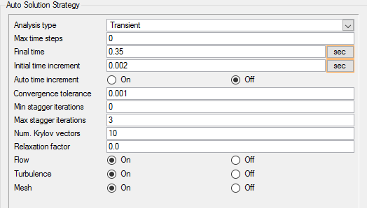
Figure 16.
Set Material Model Attributes
AcuConsole has three pre-defined materials, Air, Aluminum, and Water.
In the next steps you will verify that the pre-defined material properties of water match the desired properties for this problem.
Figure 17.
-
Double-click Material Model
in the Data Tree to expand it.
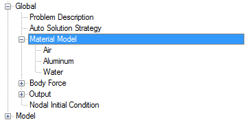
Figure 18. -
Save the database to create a backup
of your settings. This can be achieved with any of the following
methods.
- Click the File menu, then click Save.
- Click
 on
the toolbar.
on
the toolbar. - Click Ctrl+S.
Note: Changes made in AcuConsole are saved into the database file (.acs) as they are made. A save operation copies the database to a backup file, which can be used to reload the database from that saved state in the event that you do not want to commit future changes. -
Save the database to create a backup
of your settings. This can be achieved with any of the following
methods.
- Click the File menu, then click Save.
- Click on
the toolbar.
- Click Ctrl+S.
Note: Changes made in AcuConsole are saved into the database file (.acs) as they are made. A save operation copies the database to a backup file, which can be used to reload the database from that saved state in the event that you do not want to commit future changes.
Import the Geometry and Define the Model
Import the Check Valve Geometry
-
Select pressureCheckValve.x_t and click
Open to open the Import Geometry
dialog.
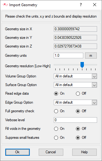
Figure 19.For this tutorial, the default values for the Import Geometry dialog are used to load the geometry. If you have previously used AcuConsole, be sure that any settings that you might have altered are manually changed to match the default values shown in the figure. With the default settings, volumes from the CAD model are added to a default volume group. Surfaces from the CAD model are added to a default surface group. You will work with groups later in this tutorial to create new groups, set flow parameters, add geometric components, and set meshing parameters.
-
Click Ok to complete
the geometry import.

Figure 20.The color of objects shown in the modeling window in this tutorial and those displayed on your screen may differ. The default color scheme in AcuConsole is "random," in which colors are randomly assigned to groups as they are created. In addition, this tutorial was developed on Windows. If you are running this tutorial on a different operating system, you may notice a slight difference between the images displayed on your screen and the images shown in the tutorial.
Create Multiplier Function for Inlet Pressure
AcuSolve provides the ability to scale values as a function of time and/or time step during a simulation. This is achieved through the use of a multiplier function. In this tutorial, the inlet stagnation pressure varies as the simulation progresses. By taking advantage of multiplier functions, you can easily set up a function to model the pressure changes at the inlet.
In the next steps you will create a multiplier function for the pressure at the inlet. This multiplier function will be applied to the inlet later in this tutorial.
Figure 21.
To make the creation of the multiplier functions as simple as possible, you will use the PB* filter in the Data Tree Manager.
-
Click PB* in the Data Tree Manager
to show all problem-definition settings.
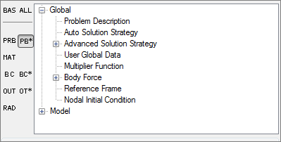
Figure 22. -
Check that the Evaluation type is set to Per Time Step.
This value indicates that AcuSolve should evaluate the multiplier function once for each time step.
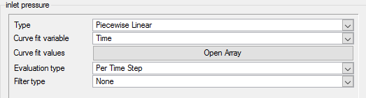
Figure 23. -
Add the function values for the inlet pressure
profile.
-
Enter the following values for X (time) and Y
(pressure).
X Y 0.0 0.0 0.002 0.0 0.05 26500 0.2 26500 0.25 0.0 0.35 0.0 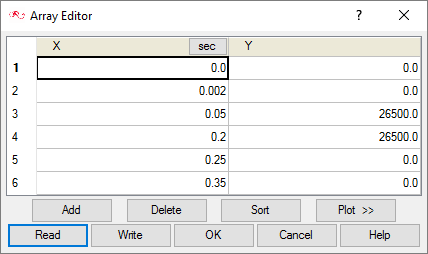
Figure 24. -
Click Plot to expand the
Array Editor dialog to display the plot of the
curve fit values.
You may need to expand the dialog by dragging the right edge in order to see the plot.
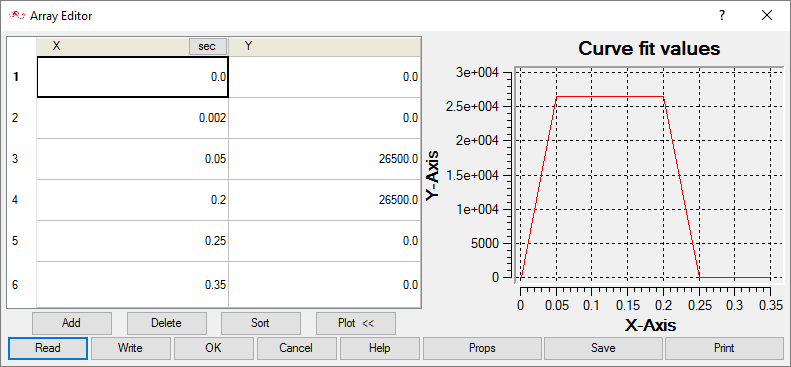
Figure 25.
These entries will be used to control the change in inlet pressure throughout the simulation. -
Enter the following values for X (time) and Y
(pressure).
Create Mesh Motion
AcuSolve uses the mesh-motion settings to define the movement of nodes within the model. In this tutorial, you will use a special case of this command that solves the dynamic equations of motion to determine the motion of the nodes. This type of mesh motion is referred to as a rigid-body dynamic. In this simulation, you will specify two inputs to define the behavior of the rigid body; the mass of the valve shutter and the stiffness of the spring that resists the movement of the valve shutter.
- Create the mesh-motion definition (this set of steps).
- Assign the mesh-motion instance to a surface group.
- Revisit the mesh-motion settings to couple the forces on the surface with the displacement of the body.
In the next steps you will create a mesh motion of type rigid body to simulate the valve shutter and virtual spring. This mesh motion defines how the valve responds to the flow forces. To simplify this task, you will use the FSI filter in the Data Tree Manager. The FSI filter limits the options in the to show only the settings related to fluid-structure interactions.
-
Define the stiffness of the virtual spring supporting the shutter.
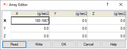
Figure 26. -
Click OK.
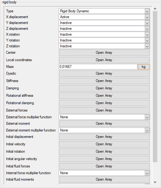
Figure 27.
Apply Volume Parameters
Volume groups are containers used for storing information about volumes. This information includes the list of geometric volumes associated with the container, as well as attributes such as material models and mesh sizing information.
When the geometry was imported into AcuConsole, all volumes were placed into the "default" volume container.
In the next steps you will rename the default volume group and set the material for the volume as water.
-
Click the drop-down control next to Material model and select
Water
Figure 28.
Create Surface Groups and Apply Surface Attributes
Surface groups are containers used for storing information about a surface. This information includes the list of geometric surfaces associated with the container, as well as attributes such as boundary conditions, surface outputs, and mesh sizing information.
In the next steps you will define surface groups, assign the appropriate attributes for each group in the problem, and add surfaces to the groups.
Set Inflow Boundary Conditions for the Inlet
In the next steps you will define a surface group for the inlet, assign the multiplier function to describe the transient pressure, and add the inlet from the geometry to the surface group.
-
Set the Turbulence viscosity ratio to 10.
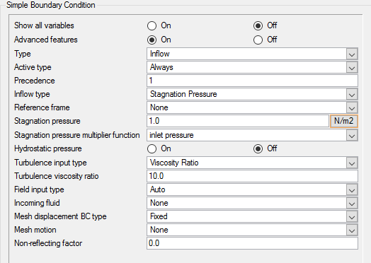
Figure 29. -
Add a geometry surface to the Inlet group.
-
Click the inlet face.
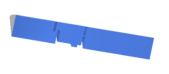
Figure 30.At this point the inlet should be highlighted
-
Click the inlet face.
Set Outflow Boundary Conditions for the Outlet
In the next steps you will define a surface group for the outlet, assign the appropriate attributes and add the outlet from the geometry to the surface group.
- Create a new surface group.
- Rename the surface to Outlet.
- Expand the Outlet surface in the tree.
- Double-click Simple Boundary Condition to open the detail panel.
- Change the Type to Outflow.
-
Add a geometry surface to the Outlet surface
container.
-
Click on the outlet face.
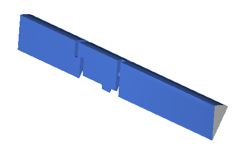
Figure 31.At this point, the outlet should be highlighted.
-
Click on the outlet face.
Set Symmetry Boundary Conditions for the Symmetry Planes
The problem is rotationally periodic, allowing for modeling with the use of a section. For this tutorial, a 30-degree section of the geometry is modeled. In order to take advantage of this, the front and rear faces of the section can be identified as symmetry planes, because the non-streamwise flow contribution is minimal. The symmetry boundary condition enforces constraints such that the flow field from one side of the plane is a mirror image of that on the other side.
In the next steps you will define a surface group for the symmetry plane on the front of the modeled section, and then create a second surface group for the back symmetry plane.
-
Turn off the display of all surface items except Front symmetry and
default.
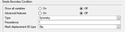
Figure 32. -
Add geometry surfaces to this group.
-
Click the symmetry plane near the inlet and near the outlet.
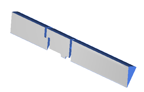
Figure 33.At this point, the front symmetry plane should be highlighted.
-
Click the symmetry plane near the inlet and near the outlet.
-
Change the Mesh displacement BC type to Slip.
This allows the mesh to move freely along the plane.
Figure 34. -
Add geometry surfaces to this group.
-
Click the symmetry plane near the inlet and near the outlet.
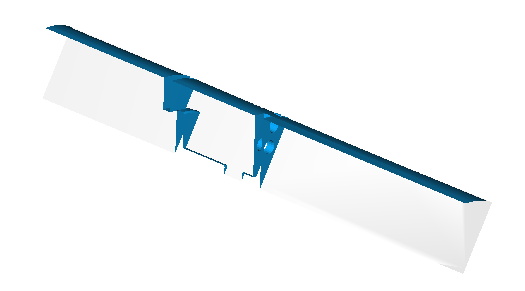
Figure 35.At this point, the back symmetry plane should be highlighted.
-
Click the symmetry plane near the inlet and near the outlet.
Set Wall Boundary Conditions for the Valve Shutter Walls
In the next steps you will define a surface group for the walls of the valve shutter, assign the appropriate settings, and add the faces from the geometry to the surface group. As part of the definition, you will assign the rigid-body mesh motion that you defined earlier to this surface.
-
Set Mesh motion to use the rigid body mesh motion that
you defined earlier in this tutorial.
-
Click rigid body.
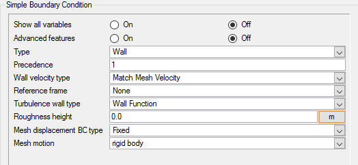
Figure 36.
-
Click rigid body.
-
Restore the initial view by clicking
 on the View Manager toolbar.
The wall of the valve is comprised of many surfaces in the geometry. By orienting the geometry properly, you can select the surfaces that make up the valve wall with the use of the "rubber band" selection tool in AcuConsole.
on the View Manager toolbar.
The wall of the valve is comprised of many surfaces in the geometry. By orienting the geometry properly, you can select the surfaces that make up the valve wall with the use of the "rubber band" selection tool in AcuConsole. -
Zoom in on the portion of the geometry that represents the valve shutter and
stem by using the right-mouse button or
 on
the View Manager toolbar.
on
the View Manager toolbar.
-
Rotate the view by left-clicking above the model and dragging the cursor down
and to the right to expose the shutter and stem walls.
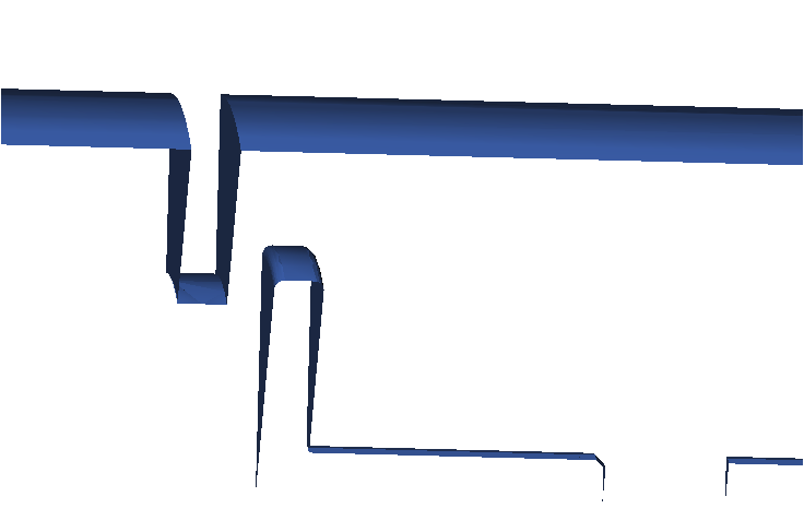
Figure 37. -
Add geometry surfaces to this group.
-
Hold the Shift key down, left-click, and drag a
selection box (rubber band) around the valve and stem.
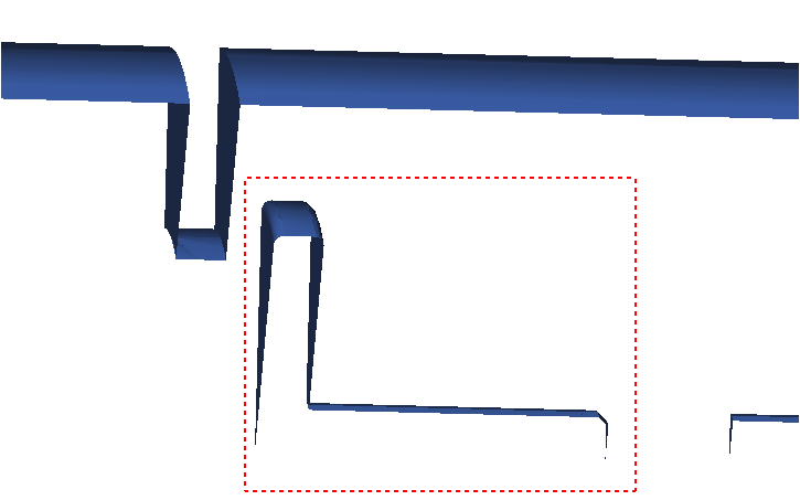
Figure 38. -
Release the left key and the valve shutter and stem should be
highlighted.
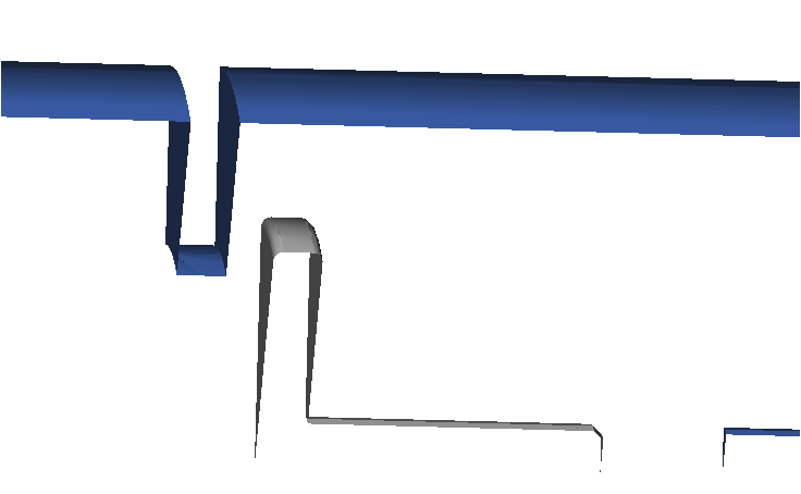
Figure 39.
-
Hold the Shift key down, left-click, and drag a
selection box (rubber band) around the valve and stem.
Set Wall Boundary Conditions for the Pipe Walls
When the geometry was loaded into AcuConsole, all geometry surfaces were placed in the default surface group. In the previous steps, you selected geometry surfaces to be placed in the groups that you created. At this point, all that is left in the default surface group is the pipe wall. Rather than create a new container, add the wall surfaces in the geometry to it, and then delete the default surface container, you will rename the existing container.
-
Double-click Simple Boundary
Condition under Pipe wall to open the detail panel.
The default wall settings will be used for the pipe wall.
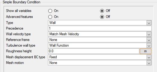
Figure 40.
Couple Mesh Motion to the Valve Wall
As the final step in enabling the use of mesh motion, you will revisit the mesh-motion definition to couple the mesh motion that you created earlier with the valve wall surface group. This step instructs AcuSolve to extract the forces on the valve from the set of surfaces that you specify in this step.
-
Click the drop-down control for row 1 and select Valve
wall.
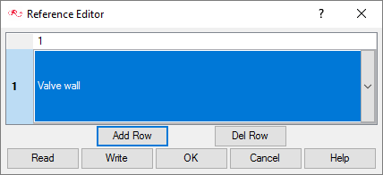
Figure 41.
Set Nodal Output Frequency
In the next steps you will set an attribute that impacts how often results from the transient simulation are written to disk. Writing the results every three time steps produces a collection of output states that can be used to create an animation of the simulation once the run has completed. Note that more frequent output can be used, but it will result in higher disk space usage.
-
Enter 3 as the Time step frequency.
This value indicates that AcuSolve should write results after every three time steps.
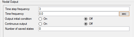
Figure 42.
Assign Mesh Controls
Set Global Meshing Parameters
Now that the simulation has been defined, attributes need to be added to define the mesh sizes that will be created by the mesher.
- Global mesh controls apply to the whole model without being tied to any geometric component of the model.
- Zone mesh controls apply to a defined region of the model, but are not associated with a particular geometric component.
- Geometric mesh controls are applied to a specific geometric component. These controls can be applied to volume groups, surface groups, or edge groups.
In the next steps you will set global meshing attributes. In subsequent steps you will create zone and surface meshing attributes.
-
Set the Maximum sweep angle to 30.0 degrees.
This option allows you to set the maximum sweep angle for edge-blend meshing on a global basis, which creates a radial array of elements around sharp edges to provide better resolution of the flow features. The sweep angle is used to control how many degrees each radial division spans.
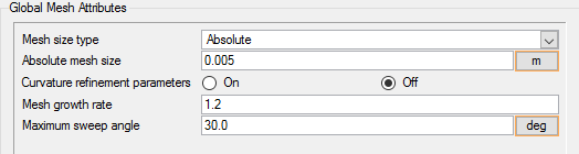
Figure 43.
Set Zone Meshing Parameters
In addition to setting meshing characteristics for the whole problem, you can assign meshing attributes to a zone within the problem where you want to be able to resolve flow with a mesh that is more refined than the global mesh. A zone mesh refinement can be created using basic shapes to control the mesh size within that shape. These types of mesh refinement are used when refinement is needed in an area that does not correspond to a geometric item.
In the following steps you will add mesh refinements in the zone around the valve gap and around the valve body.
Set Zone Meshing Parameters for the Gap
In the next steps you will add a set of mesh attributes for a zone around the gap between the valve shutter and the orifice.
-
Restore the initial view by clicking on
the View Manager toolbar.
-
Enter 0.0015 m for the Mesh size.
This will result in a zone where the mesh size provides at least three cells between the shutter and the edge of the orifice in the initial position.
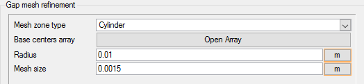
Figure 44.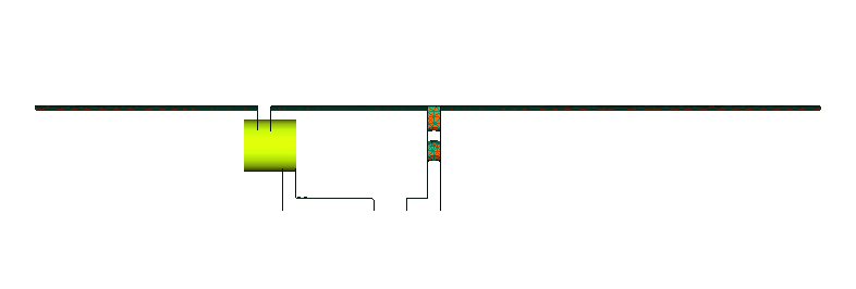
Figure 45.
Set Zone Meshing Parameters for the Valve Body
In the next steps you will add a set of mesh attributes for a zone around the valve body.
-
Enter 0.0025 m for the Mesh size.
This will result in a zone where the mesh size is half of the global mesh size.
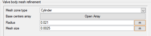
Figure 46.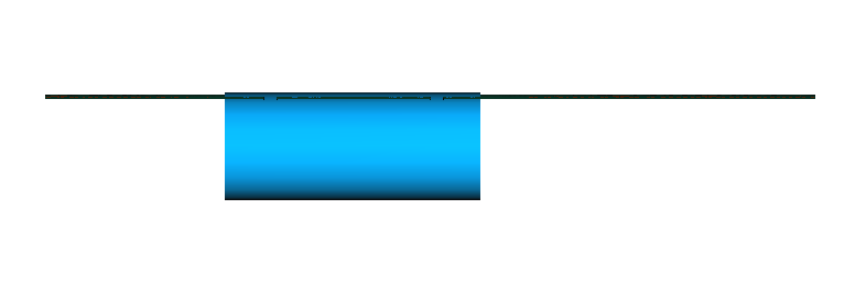
Figure 47.
Set Meshing Attributes for Surface Groups
In the following steps you will set meshing attributes that will allow for localized control of the mesh size on surface groups that you created earlier in this tutorial. Specifically, you will set local meshing attributes that control the growth of boundary layer elements normal to the surfaces of the pipe walls and valve walls.
Set Surface Meshing Attributes for the Pipe Walls
In the next steps you will set meshing attributes that allow for localized control of the mesh near the walls of the pipe. The mesh size on the wall of the pipe will be inherited from the global mesh size that was defined earlier. The settings that follow will only control the growth of the boundary layer from the walls of the pipe into the fluid volume.
-
Enter 30.0 degrees as the Maximum sweep angle.
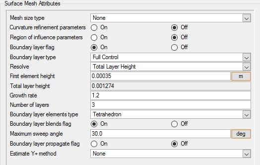
Figure 48.
Set Surface Meshing Attributes for the Valve Walls
In the next steps you will set meshing attributes that allow for localized control of the mesh size near the walls of the valve shutter assembly.
-
Enter 30.0 degrees as the Maximum sweep angle.
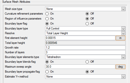
Figure 49.
Generate the Mesh
In the next steps you will generate the mesh that will be used when computing a solution for the problem.
-
Click
 on the toolbar to open the Launch
AcuMeshSim dialog.
For this case, the default values will be used.
on the toolbar to open the Launch
AcuMeshSim dialog.
For this case, the default values will be used. -
Click Ok to begin
meshing.
During meshing an AcuTail window opens. Meshing progress is reported in this window. A summary of the meshing process indicates that the mesh has been generated.
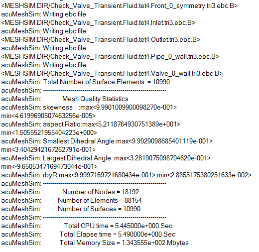
Figure 50. -
Turn off the display of Gap mesh refinement and Valve wall mesh refinement
under by clicking
 next to the surface so that it is in the display off
state (
next to the surface so that it is in the display off
state ( ),
),
Details of the mesh on the front symmetry plane are shown in Figure 51. This view was obtained by reorienting the view with
on the View Manager toolbar, then zooming in on the
model.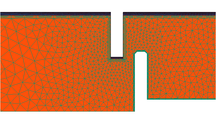
Figure 51. Mesh Details Around the Valve Viewed on the Front Symmetry PlaneNote that the mesh size in the pipe decreases from left to right in the transition from a region where global settings determine the size to the zone around the gap where the settings are for a finer mesh. Note also that the mesh to the right of the valve shutter is smaller than the global mesh as determined in the Valve body mesh refinement that you created.
Compute the Solution and Review the Results
Run AcuSolve
In the next steps you will launch AcuSolve to compute the solution for this case.
-
Click
 on the toolbar to open the
Launch AcuSolve dialog.
on the toolbar to open the
Launch AcuSolve dialog.
-
Click Ok to start the
solution process.
While computing the solution, an AcuTail window opens. Solution progress is reported in this window. A summary of the solution process indicates that the run has been completed.
The information provided in the summary is based on the number of processors used by AcuSolve. If you use a different number of processors than indicated in this tutorial, the summary for your run may be slightly different than the summary shown.
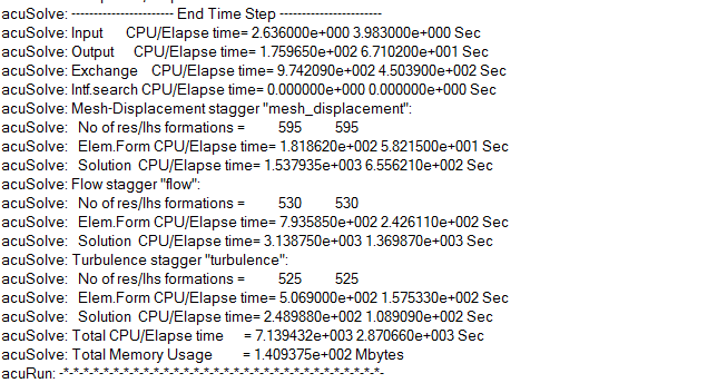
Figure 52.
Monitor the Solution with AcuProbe
While AcuSolve is running, you can monitor the inlet pressure and displacement of the valve using AcuProbe.
-
Open AcuProbe by clicking
 on the toolbar.
-
Right-click on pressure and select
Plot.
As the solution progresses, the plot will update. If you opened AcuProbe after the solution completed, click
 to refresh the plot.
 -
Right-click on
mesh_x_displacement and select
Plot.
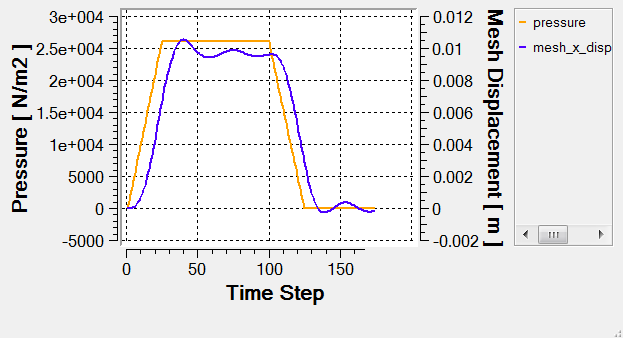
Figure 53.
Post-Process Flow Rate with AcuProbe
In the next steps you will create a user function for the display of volume flow rate in AcuProbe.
-
Create a user function for volume flow rate.
-
Click
 on the toolbar to open the User
Function dialog.
on the toolbar to open the User
Function dialog.
-
On the next line, type value =
mass_flux/1000.0.
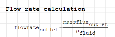
This sets the value to be plotted as the mass flux at the outlet divided by the density of water.
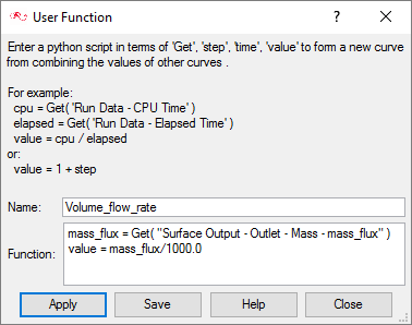
Figure 54.
-
Click
-
Click on the toolbar to refresh the plot of volume flow
rate.
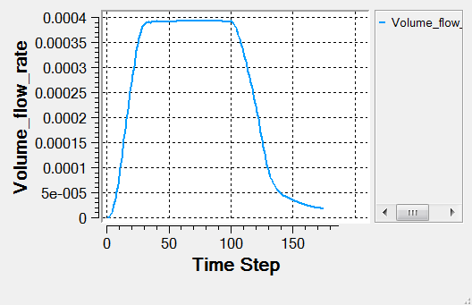
Figure 55.
View Results with AcuFieldView
Now that a solution has been calculated, you are ready to view the flow field using AcuFieldView. AcuFieldView is a third-party post-processing tool that is tightly integrated toAcuSolve. AcuFieldView can be started directly from AcuConsole, or it can be started from the Start menu, or from a command line. In this tutorial you will start AcuFieldView from AcuConsole after the solution is calculated by AcuSolve.
In the following steps you will start AcuFieldView, display velocity magnitude and animate the view to show mesh displacement. You will then display velocity vectors and pressure contours when the valve shutter is at maximum displacement.
Start AcuFieldView
-
Click
 on the
AcuConsole toolbar to open the
Launch AcuFieldView dialog.
on the
AcuConsole toolbar to open the
Launch AcuFieldView dialog.
Display Velocity Magnitude on the Front Symmetry Plane
In the next steps you will create a boundary surface to display contours of velocity magnitude on the front symmetry plane of the modeled slice.
These steps are provided with the assumption that you are able to manipulate the view in AcuFieldView to have a white background, perspective turned off, outlines turned off, and the viewing direction set to +Z. If you are unfamiliar with basic AcuFieldView operations, refer to Manipulate the Model View in AcuFieldView .
-
Click
 to open the Boundary
Surface dialog.
Note: The dialog may already be open. This step will put the focus on the dialog.
to open the Boundary
Surface dialog.
Note: The dialog may already be open. This step will put the focus on the dialog. -
Add a legend to the view.
- Click the Legend tab in the Boundary Surface dialog.
- Enable the Show Legend option.
- Enable the Frame option.
- Click the white color swatch next to Geometric in the Color group and set the color for the legend values to black.
- Set Decimal Places to 1.
- Click the white color swatch next to the Title field and set the color for the title to black.
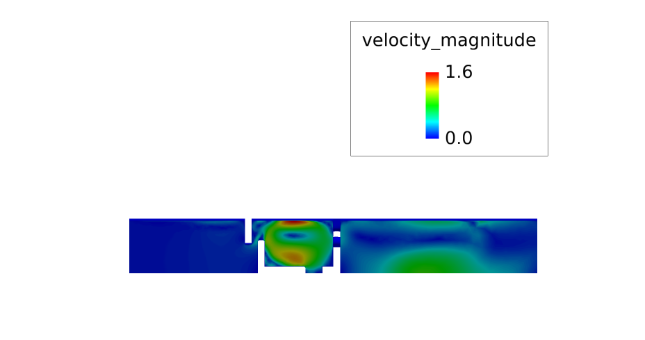
Figure 56.This image was created with a white background, perspective turned off, outlines turned off, and the viewing direction set to +Z.
When data was loaded from AcuSolve, AcuFieldView displays information from the final time step. In the following steps you will display velocity magnitude at the first time step and then animate the display to show the motion of the valve shutter and the velocity changes throughout the simulation.
Animate the Display of Velocity Magnitude
In the next steps you will create a transient sweep and save it as an animation that can be viewed independently of AcuFieldView. As a first step, you will change the colormap used by the legend.
-
Set the colormap to use defined maximum and minimum
values throughout the transient sweep.
- Click the Colormap tab.
- Enter 6.6 for the maximum.
- Enter 0 for the minimum.
These settings will be used throughout the transient sweep so that the contours at each time step will all be relative to this specified range.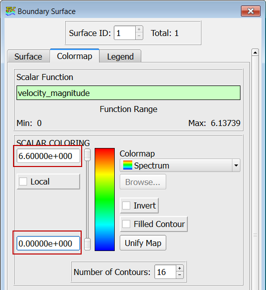
Figure 57. -
Click OK to dismiss
the Flipbook Size Warning dialog.
The Sweep button on the Transient Data Controls dialog will have changed to Build.
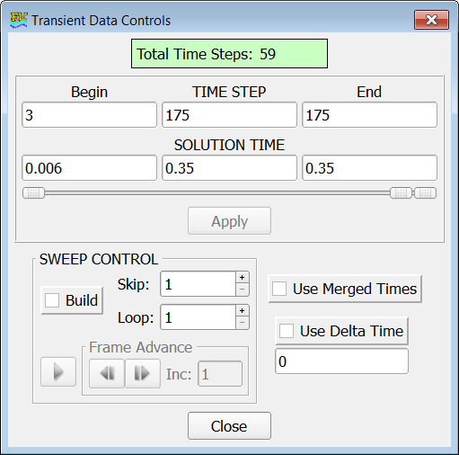
Figure 58. -
Click Build.
As AcuFieldView builds the flipbook animation, you will see the controls on the Transient Data Controls dialog advance. Once the flipbook is built, a Flipbook Controls dialog will allow you to play or save the animation.
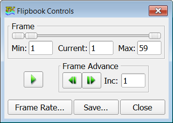
Figure 59.
Display Pressure Contours and Velocity Vectors on a Mid-Z Coordinate Surface
In the next steps you will create a coordinate surface at the mid-Z plane of the modeled section. You will then display pressure contours and velocity vectors on that surface.
-
Click
 to open
the Coordinate Surface dialog.
to open
the Coordinate Surface dialog.
-
Create a second coordinate surface at the mid-Z
plane for the display of velocity vectors.
-
Click Create on
the Surface tab of the Coordinate Surface
dialog.
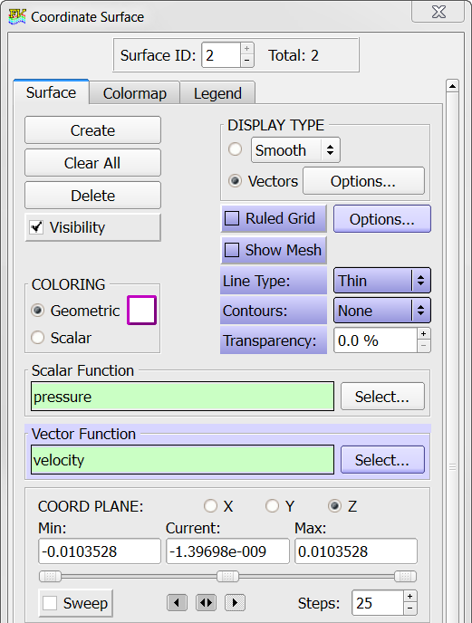
Figure 60. -
Click Options next to Vectors.
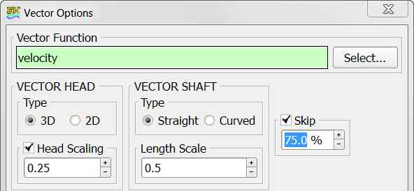
Figure 61.
-
Click Create on
the Surface tab of the Coordinate Surface
dialog.
-
Set transient data to display the
78th time step.
- Open .
- Use the slider to set the Time Step to 78.
- Click Apply.
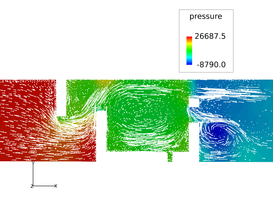
Figure 62.
Summary
In this tutorial, you worked through a basic workflow to set up a transient simulation with a moving mesh and variable inlet pressure. Once the case was set up, you generated a mesh and generated a solution using AcuSolve. AcuProbe was used to post-process the motion of the valve shutter (x_mesh_displacement) and to calculate volume flow at the outlet. Results were also post-processed in AcuFieldView to allow you to create contour and vector views, and to allow you to view the transient data. New features introduced in this tutorial include: transient simulation, multiplier functions, mesh motion, post-processing with AcuProbe, and animation of transient results.