ACU-T: 4002 Sloshing of Water in a Tank
Prerequisites
This tutorial provides instructions for running a transient simulation of a two-phase flow in a rectangular tank using the level set model. Prior to starting this tutorial, you should have already run through the introductory HyperWorks tutorial, ACU-T: 1000 HyperWorks UI Introduction, and have a basic understanding of HyperWorks CFD and AcuSolve. To run this simulation, you will need access to a licensed version of HyperWorks CFD and AcuSolve.
Prior to running through this tutorial, copy HyperWorksCFD_tutorial_inputs.zip from <Altair_installation_directory>\hwcfdsolvers\acusolve\win64\model_files\tutorials\AcuSolve to a local directory. Extract ACU-T4002_TankSloshing.hm and bodyForce.c from HyperWorksCFD_tutorial_inputs.zip.
Since the HyperWorks CFD database (.hm file) contains meshed geometry, this tutorial does not include steps related to geometry import and mesh generation.
Problem Description
The problem to be solved is shown schematically in the figure below. It consists of a partially filled water tank and from time t=0, water inside the tank is subjected to a sinusoidal varying body force along x-direction and constant gravity along y-direction.

Figure 1.
The body force in the x-direction is given by the expression:
- Α = Amplitude of oscillation = -0.06 m
- ω = Frequency of oscillation = = 3.6 rad/sec
- T = Time period of oscillation = 1.74 sec
- φ = Phase difference = 0
Start HyperWorks CFD and Open the HyperMesh Database
-
From the Home tools, Files tool group, click the Open Model tool.

Figure 2.The Open File dialog opens.
Validate the Geometry
The Validate tool scans through the entire model, performs checks on the surfaces and solids, and flags any defects in the geometry, such as free edges, closed shells, intersections, duplicates, and slivers.
Figure 3.
Set Up the Problem
Set Up the Simulation Parameters and Solver Settings
-
From the Flow ribbon, click the Physics tool.

Figure 4.The Setup dialog opens. -
Under the Physics models setting:
- Activate the Multiphase flow radio button.
- Set the Multifluid type to Immiscible and the Immiscible material to Air-Water
- Set the Time step size to 0.006 and the Final time to 4.0
- Select Laminar as the Turbulence model.
- Set the gravity to -9.81 m/sec2 in the y direction.
- Select Absolute for the Pressure scale.
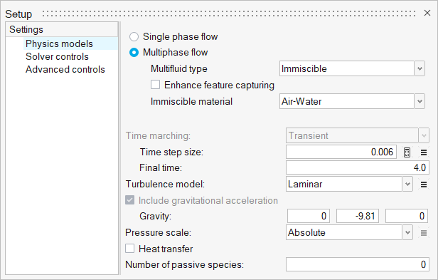
Figure 5. -
Click the Solver Controls setting.
- Set the Minimum stagger iterations to 2.
- Set the Maximum stagger iterations to 6.
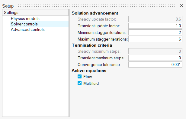
Figure 6.
Assign Material Properties
-
From the Flow ribbon, click the Material tool.

Figure 7. -
Click
 on the guide bar.
Set the Body Force
-
From the Flow ribbon, click the tool.

Figure 8. -
Click
 and enter the following
values.
and enter the following
values.
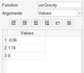
Figure 9.These values are for the amplitude of oscillation = -0.06 m; time period of oscillation = 1.74 sec; Phase difference = 0
-
On the guide bar, click
 to execute
the command and exit the tool.
to execute
the command and exit the tool.
Compile the Body Force UDF
-
For Windows:
-
For Linux:
Define Flow Boundary Conditions
-
From the Flow ribbon, click the No Slip tool.

Figure 10. -
Select all four surfaces shown in the figure below.
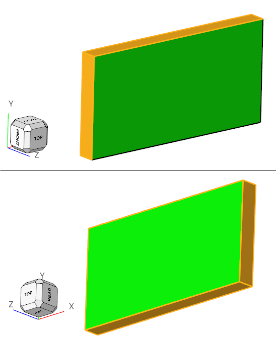
Figure 11. -
Click on the guide bar.
-
Click the Slip tool.

Figure 12. -
Select the right most face on the positive z-axis, as shown in the figure
below.
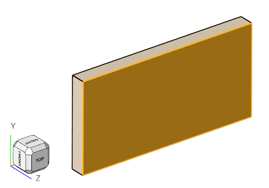
Figure 13. -
On the guide bar, click
 to execute the command and remain in the
tool.
to execute the command and remain in the
tool.
-
Click on the guide bar.
Define Nodal Initial Conditions
-
From the Solution ribbon, click the
Plane tool.

Figure 14. -
Click
 in the microdialog and
manually set the plane axis to Y.
in the microdialog and
manually set the plane axis to Y.
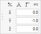
Figure 15. -
Click
 and set the coordinates to (0.60, 0.12,
0.10).
and set the coordinates to (0.60, 0.12,
0.10).
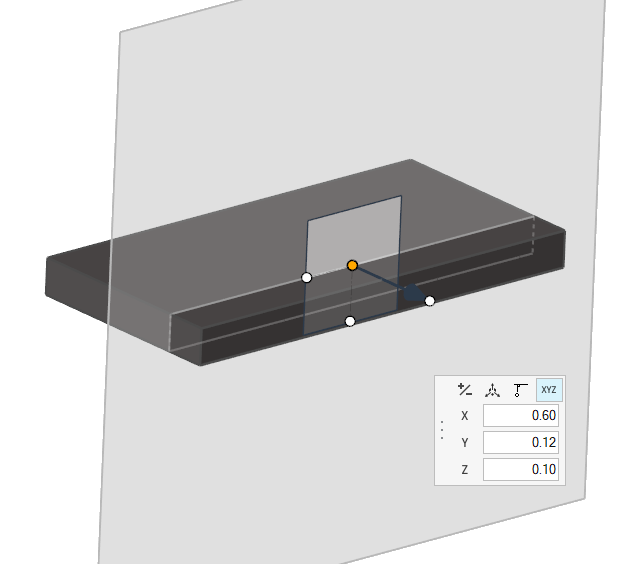
Figure 16. -
Click
 to add a variable then select Fluid from the
list.
to add a variable then select Fluid from the
list.
-
Make sure that the Value is set to Water then press
Esc again.
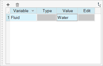
Figure 17. -
Click on the guide bar.
Define Nodal Outputs
-
From the Solution ribbon, click the Field tool.

Figure 18.The Field Output dialog opens. -
Set the parameters for Solution variables as shown in the figure below.
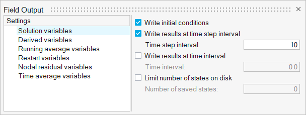
Figure 19.
Run AcuSolve
-
From the Solution ribbon, click the Run tool.

Figure 20.The Launch AcuSolve dialog opens. -
Leave the remaining options as default and click
Run to launch AcuSolve.
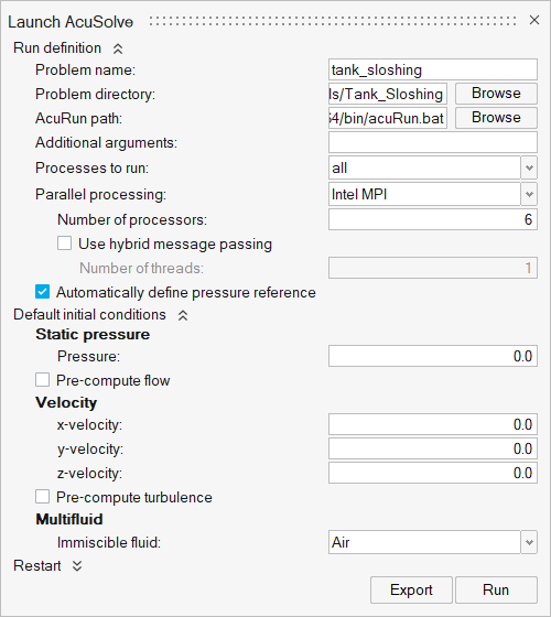
Figure 21.The Run Status dialog opens. Once the run is complete, the status is updated and you can close the dialog.Tip: While AcuSolve is running, right-click on the AcuSolve job in the Run Status dialog and select View Log File to monitor the solution process.
Post-Process the Results with HW-CFD Post
-
Click the Top face on the View Cube to align the
model.
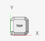
Figure 22. -
Activate the Legend toggle and click
 to refresh the range.
-
Click
 , and set the Colormap Name to Rainbow
Uniform.
, and set the Colormap Name to Rainbow
Uniform.
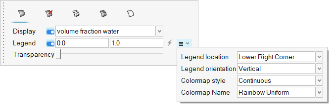
Figure 23. -
Click on the guide bar.
-
Click
 at the bottom of the modeling window to view a live animation of the flow.

Figure 24. -
Save the animation.
- Go to .
-
Click
 on the toolbar.
- Uncheck Include mouse cursor.
- Set the frame rate to 24.
-
Click
 on the toolbar then drag over the area you
want to record.
on the toolbar then drag over the area you
want to record.
-
Click
 to start recording and the same button to
stop recording.
to start recording and the same button to
stop recording.
- Name the file and save it.
Summary
In this tutorial, you successfully learned how to set up and solve a transient multiphase flow problem involving water sloshing in a tank using HyperWorks CFD and AcuSolve. You also learned how to create a multiphase model using the Level Set method and specify the body force using a user-defined function and then compile the UDF. Once the solution was computed, you post-processed the results using the Post ribbon where you generated an animation of the water sloshing in the tank.