ACU-T: 3400 AcuSolve-Flux Integration
This tutorial provides instructions for setting up, solving, and viewing results for simulation of a 2D cable for simple conduction analysis. In this simulation, the heated solid volume is used for conduction with the outer volume and comes with a flux value already calculated using another software. This tutorial is designed to introduce you to a new feature, the Electromagnetics Manager, wherein the flux is imported on to the heated volume in the form of a Nastran file.
- Importing the heat flux using the Electromagnetics Manger in AcuConsole
- Mesh extrusion from one surface to other surface
- Use of the Variable Manager for defining all the variables in a single panel
- Post-processing with AcuFieldView for plotting temperature contours
- Creating or modifying 2D Plots in AcuFieldView
In this tutorial, you will do the following:
- Analyze the problem
- Start AcuConsole and create a simulation database
- Set general problem parameters
- Set solution strategy parameters
- Assign material properties for the solid volume
- Import the geometry for the simulation
- Create a volume group and apply volume parameters
- Create surface groups and apply surface parameters
- Set global and local meshing parameters
- Generate the mesh
- Set the appropriate boundary conditions
- Import Nastran file using the Electromagnetics Manager for importing Flux
- Run AcuSolve
- Monitor the solution with AcuFieldView
Prerequisites
You should have already run through the introductory tutorial, ACU-T: 2000 Turbulent Flow in a Mixing Elbow. It is assumed that you have some familiarity with AcuConsole, AcuSolve, and AcuFieldView. You will also need access to a licensed version of AcuSolve.
Prior to running through this tutorial, copy AcuConsole_tutorial_inputs.zip from <Altair_installation_directory>\hwcfdsolvers\acusolve\win64\model_files\tutorials\AcuSolve to a local directory. Extract 2DCable.x_t and CABLE_EXAMPLE_MOD.nas from AcuConsole_tutorial_inputs.zip.
Analyze the Problem
An important step in any CFD simulation is to examine the engineering problem at hand and determine the important parameters that need to be provided to AcuSolve. Parameters can be based on geometrical elements, such as inlets, outlets, or walls, and on flow conditions, such as fluid properties, velocity, or whether the flow should be modeled as turbulent or as laminar.
Figure 1 shows a simple 2D cable problem wherein the inner cylinder is provided with a volumetric heat source of 1.46686 W and is in contact with the outer cylinder, the outer surface of which is maintained at a temperature of 20oC (293K).This problem forms the basis of a simple conduction analysis between two concentric cylinders. The only difference from the basic problem is that the heat source is calculated using another software called Flux and is provided using AcuConsole’s EMag (Electromagnetic) Manger to account for volumetric losses from Flux to AcuSolve.

Figure 1.
- Fluid rotational effects
- Material specific properties (temperature dependent, non-Newtonian)
- Convection on the outer surface
Coupling of AcuSolve to Flux will also enable the inclusion of natural convection and forced convection effects into the thermal calculation of various electrical devices.
Define the Simulation Parameters
Start AcuConsole and Create the Simulation Database
In this tutorial, you will begin by creating a database, populating the geometry-independent settings, loading the geometry, creating volume and surface groups, setting group parameters, adding geometry components to groups, and assigning mesh controls and boundary conditions to the groups. Next you will generate a mesh and run AcuSolve to solve for the number of time steps specified. Finally, you will visualize some characteristics of the results using AcuFieldView.
In the next steps you will start AcuConsole, and create the database for storage of the simulation settings.
-
Click the File menu, then click
New to open the New data
base dialog.
Note: You can also open the New data base dialog by clicking
 on the toolbar.
Set General Simulation Parameters
In next steps you will set parameters that apply globally to the simulation. To make this simple, the basic settings applicable for any simulation can be filtered using the BAS filter in the Data Tree Manager. This filter enables display of only a small subset of the available items in the Data Tree and makes navigation of the entries easier.
-
Click BAS in the Data Tree Manager to switch to basic view in the Data Tree.
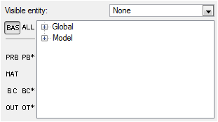
Figure 2. -
Double-click the Global
Data Tree item to expand it.
Tip: You can also expand a tree item by clicking
 next to the item name.
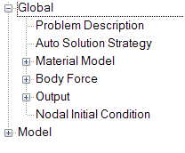
Figure 3. -
Set Abs. temperature offset to 0 K.

Figure 4.
Set Solution Strategy Parameters
In the next steps you will set parameters that control the behavior of AcuSolve as it progresses during the solution.
-
Set the Flow flag to Off.
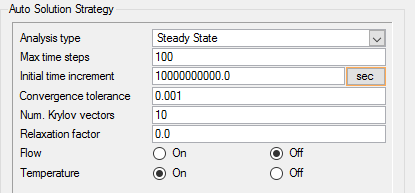
Figure 5.
Set Material Model Parameters
-
Double-click Material Model
in the Data Tree to expand it.
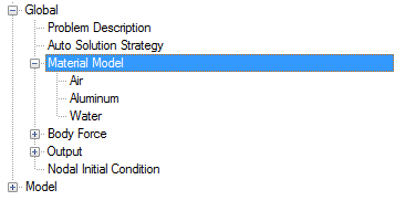
Figure 6. -
Save the database to create a backup
of your settings. This can be achieved with any of the following
methods.
- Click the File menu, then click Save.
- Click
 on
the toolbar.
on
the toolbar. - Click Ctrl+S.
Note: Changes made in AcuConsole are saved into the database file (.acs) as they are made. A save operation copies the database to a backup file, which can be used to reload the database from that saved state in the event that you do not want to commit future changes.
Import the Geometry and Define the Model
Import the Geometry
-
Select 2DCable.x_t and click
Open to open the Import Geometry
dialog.
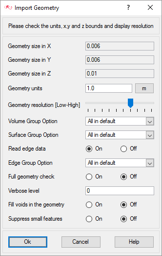
Figure 7.For this tutorial, the default values for the Import Geometry dialog are used to load the geometry. If you have previously used AcuConsole, be sure that any settings that you might have altered are manually changed to match the default values shown in the figure. With the default settings, volumes from the CAD model are added to a default volume group. Surfaces from the CAD model are added to a default surface group. You will work with groups later in this tutorial to create new groups, set flow parameters, add geometric components, and set meshing parameters.
-
Rotate the visualization to view the entire model.
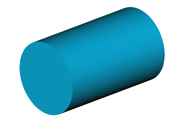
Figure 8.The color of objects shown in the modeling window in this tutorial and those displayed on your screen may differ. The default color scheme in AcuConsole is "random," in which colors are randomly assigned to groups as they are created. In addition, this tutorial was developed on Windows. If you are running this tutorial on a different operating system, you may notice a slight difference between the images displayed on your screen and the images shown in the tutorial.
Apply Volume Parameters
Volume groups are containers used for storing information about a volume region. This information includes the list of geometric volumes associated with the container, as well as attributes such as material models and mesh size information.
When the geometry was imported into AcuConsole, all volumes were placed into the "default" volume container.
In the next steps you will create volume groups for each volume in the model, assign volumes to the respective volume groups, rename the default volume group container, and set the materials and other properties for each volume group.
-
Expand Volumes. Toggle the display of the default
volume container by clicking
 and
and  next to the volume name.
Note: You may not see any change when toggling the display if Surfaces are being displayed, as surfaces and volumes may overlap.
next to the volume name.
Note: You may not see any change when toggling the display if Surfaces are being displayed, as surfaces and volumes may overlap. -
Assign the respective volumes to their volume groups.
-
Select the volume shown in the figure below and click
Done.
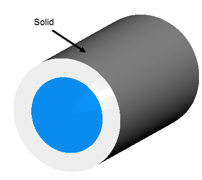
Figure 9.
-
Select the volume shown in the figure below and click
Done.
-
When the geometry was loaded into AcuConsole, the
complete geometry volume was placed in the default volume group. This default
volume group was renamed to SolidHeated. In the previous step, you assigned a
volume to the other volume group that you created. At this point, all that is
left is the SolidHeated volume group
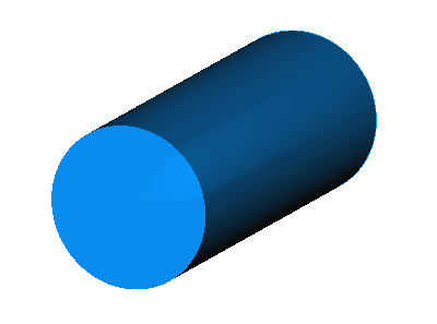
Figure 10.
Create Surface Groups and Apply Surface Parameters
Surface groups are containers used for storing information about a surface, including solution and meshing parameters, and the corresponding surface in the geometry that the parameters will apply to.
In the next steps you will define surface groups, assign the appropriate settings for the different characteristics of the problem, and add surfaces to the group containers.
-
Rename the other surfaces and set the Simple BC Active and Simple BC Type
columns as per the table shown below.
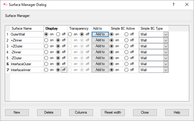
Figure 11. -
Assign the surfaces to their respective surface groups.
-
Select the planar surface shown in the figure below and click
Done.
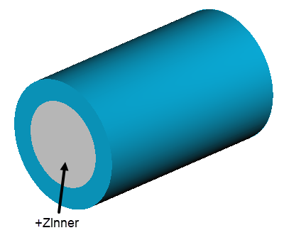
Figure 12. -
Select the planar surface shown in the figure below and click
Done.
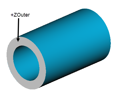
Figure 13. -
In a similar manner, select the -ZInner and -ZOuter surfaces.
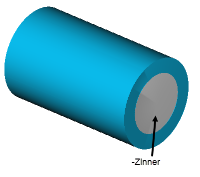
Figure 14.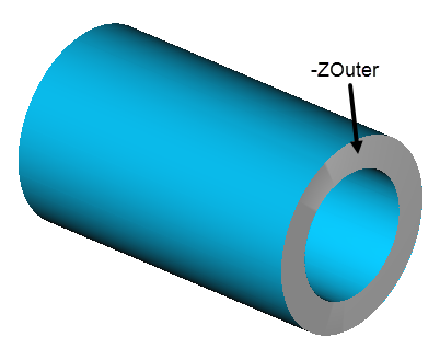
Figure 15. -
Assign the surface for InterfaceOuter.
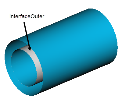
Figure 16. -
Assign the surface for InterfaceInner
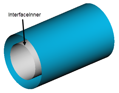
Figure 17. -
When the geometry was loaded into AcuConsole, all the geometry surfaces were placed in the default surface group
container. This default surface group was renamed to OuterWall. In the
previous steps, you assigned some surfaces to various other surface
groups that you created. At this point, all that is left is the
OuterWall surface group.
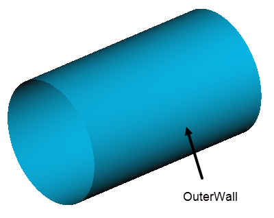
Figure 18.
-
Select the planar surface shown in the figure below and click
Done.
Assign Volume Parameters (Element Material Properties)
Solid
-
Leave the remaining parameters as it is.
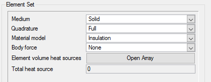
Figure 19.
SolidHeated
The SolidHeated group will have the same settings as Solid group. In order to not to repeat the step again, we can propagate the settings to that group as follows:
Assign Surface Parameters (Boundary Conditions)
In next steps, you will set boundary conditions for the surfaces that apply globally to the simulation. To make this simple, the boundary conditions applicable for any simulation can be filtered using the BC filter in the Data Tree Manager.
OuterWall
The OuterWall group defines the wall through which conduction takes place.
-
Set Temperature to 293.0 K.
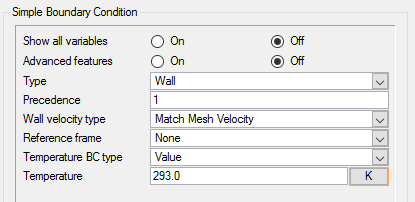
Figure 20.
Remaining Groups
-
Select all the other groups except OuterWall in the pop-up window and click
Propagate.
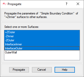
Figure 21.Note: You can ensure the settings are applied correctly by expanding the other surface group and cross checking the boundary conditions.
Define the Variables List
-
Click the Variable List icon from the main toolbar.
 Figure 22. Tip: You can also click .The Variable Manager dialog opens.
 -
Create six variables using the Name and Expression data shown below then click
Close.
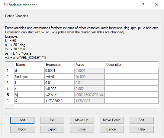
Figure 23.Note: Type equal (=) or colon equal (:=) in the Expression column before entering an expression. The expression will be valid only if either of these two symbols are used. Equal to (=) calculates the value of the expression when defined and uses it, whereas colon equal (:=) recalculates the value of the expression if any relative variable is changed.The variables L, r, V, Q denote length of the cylinder, radius, area of the cylindrical surface, and heat flux respectively.
Assign Mesh Controls
Set Global Mesh Attributes
Now that the flow characteristics have been set for the whole problem, a sufficiently refined mesh has to be generated.
Global mesh attributes are the meshing parameters applied to the model as a whole without reference to a specific geometric volume, surface, edge, or point. Local mesh attributes are used to create mesh generation controls for specific geometry components of the model.
In the next steps you will set the global mesh attributes.
-
Change the Mesh growth rate to 1.2.
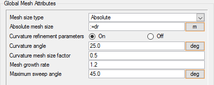
Figure 24.
Set Volume Mesh Attributes
Volume mesh attributes are the meshing parameters applied to a particular volume. You have the option to control the mesh size on a volume and define curvature refinement parameters like curvature angle and the curvature mesh size factor.
In the next steps you will set the volume mesh attributes.
-
In the detail panel, change the Absolute mesh size to
:=dr.
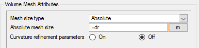
Figure 25.Note: :=dr refers to the value of the variable dr, which was defined in the Variables Manager earlier. This means that the Solid volume group has an absolute mesh size of 0.0001m.
Set Surface Mesh Attributes
Surface mesh attributes are applied to a specific surface in the model. It is a type of local meshing parameter used to create targeted mesh controls for one or more specific surfaces.
Setting local mesh attributes, such as surface mesh attributes, is not mandatory. When a local mesh attribute is not found for a component, the global attributes are used as the mesh generation control for that component. If a local mesh attribute is present, it will take precedence over the global setting.
In the next steps you will set the surface meshing attributes.
-
Set the Growth rate to 1.2.
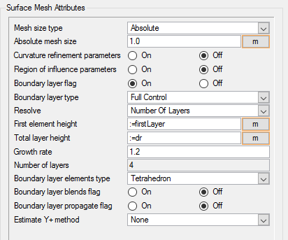
Figure 26.
Define Mesh Extrusions
Mesh extrusion is a feature that allows the generation of structured mesh in the entire volume or only on the surface. This feature extrudes the mesh on one surface to another surface and can also be used with other meshing features. In this case, we are going to extrude the mesh along the length of both the Inner and Outer cylinders from one end to the other.
Mesh Extrusion is available under the Model tree.
-
Change the Extrusion options to All tets.
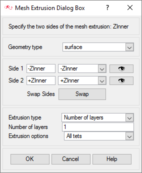
Figure 27. -
Similarly, repeat the same procedure for ZOuter. The final dialog should look
like the image below.

Figure 28.
Generate the Mesh
In the next steps you will generate the mesh that will be used when computing a solution for the problem.
-
Click
 on the toolbar to open the Launch
AcuMeshSim dialog.
For this case, the default settings will be used.
on the toolbar to open the Launch
AcuMeshSim dialog.
For this case, the default settings will be used. -
Click Ok to begin meshing.
During meshing an AcuTail window opens. Meshing progress is reported in this window. A summary of the meshing process indicates that the mesh has been generated.
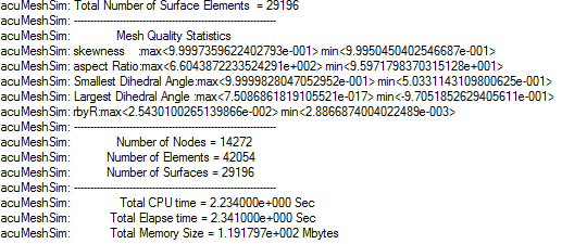
Figure 29.Note: The actual number of nodes and elements, and memory usage may vary slightly from machine to machine.
Compute the Solution and Review the Results
Transfer Heat Loss Using the Electromagnetics Manager
The Electromagnetics Manager is a tool designed for transferring the electromechanical heat losses from an EMag (Electromagnetics) output file to the appropriate element set in the CFD mesh. Flux is a simulation software used in the development and design of electrical devices. It incorporates simulation technology to accurately analyze a wide range of physical phenomena that includes complicated geometry, various material properties, and the heat and structure at the center of electromagnetic fields. The electromagnetics mesh and the element set of the CFD mesh on to which the data is transferred must have the same size and coordinates.
In this case, the heat load is already calculated from the Electromagnetics software and imported into the CFD mesh in the form of a .nas (NASTRAN) file. You do not need to calculate this value; it is provided directly with the input files. In the next steps, you will learn how to import this .nas file using the Electromagnetics Manager.
-
From the main toolbar, click the Electromagnetics Manager icon
 .
Tip: You can also click .The Electromagnetics Manager dialog opens.
.
Tip: You can also click .The Electromagnetics Manager dialog opens. -
Click Open next to Import. Select
CABLE_EXAMPLE_MOD.nas from your working directory and
click Open.
This opens the Flux Total Heat Source showing the total heat source vs time step plot and the average step data at the bottom.
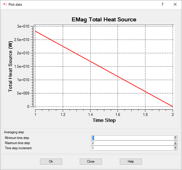
Figure 30. -
Select SolidHeated and click
OK.
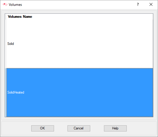
Figure 31. -
In order to confirm the heat source is correctly applied to the SolidHeated
volume group, check the Element Set.
-
Click Open Array.
The heat source is updated for the node id.
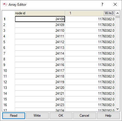
Figure 32.You can also see that the Total heat source in the Element Set detail panel is updated.
-
Click Open Array.
Run AcuSolve
In the next steps you will launch AcuSolve to compute the solution for this case.
-
Click
 on the toolbar to open the
Launch AcuSolve dialog.
on the toolbar to open the
Launch AcuSolve dialog.
-
Click Ok to start the
solution process.
While computing the solution, an AcuTail window opens. Solution progress is reported in this window. A summary of the solution process indicates that the run has been completed.
The information provided in the summary is based on the number of processors used by AcuSolve. If you use a different number of processors than indicated in this tutorial, the summary for your run may be slightly different than the summary shown.
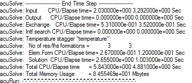
Figure 33.
View Results with AcuFieldView
Now that a solution has been calculated, you are ready to view the flow field using AcuFieldView. AcuFieldView is a third-party post-processing tool that is tightly integrated to AcuSolve. AcuFieldView can be started directly from AcuConsole, or it can be started from the Start menu, or from a command line. In this tutorial you will start AcuFieldView from AcuConsole after the solution is calculated by AcuSolve.
In the following steps you will start AcuFieldView, create a boundary surface showing temperature and plot temperature vs the radius of the model.
Launch AcuFieldView
-
Click
 on the
AcuConsole toolbar to open the
Launch AcuFieldView dialog.
on the
AcuConsole toolbar to open the
Launch AcuFieldView dialog.
Create a Boundary Surface Showing Temperature on the Surface
-
Click Viewer Options.
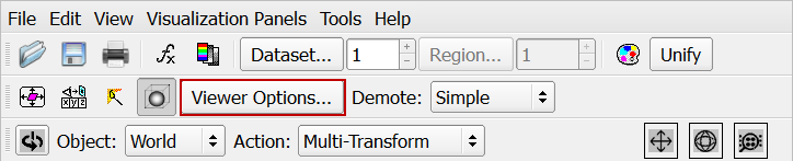
Figure 34. -
On the toolbar, click the Colormap icon
 .
.
-
Click the Toggle Outline icon
 on the toolbar to turn off the outline display.
Your display should now look like this.
on the toolbar to turn off the outline display.
Your display should now look like this.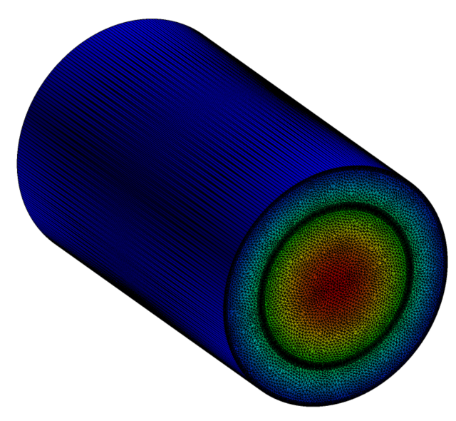
Figure 35. -
From the toolbar, click
 to open the Defined
Views dialog.
to open the Defined
Views dialog.
-
Change the Labels, Annotation, and Subtitle color to black.
Tip: You can move the legend using Shift + left-click.
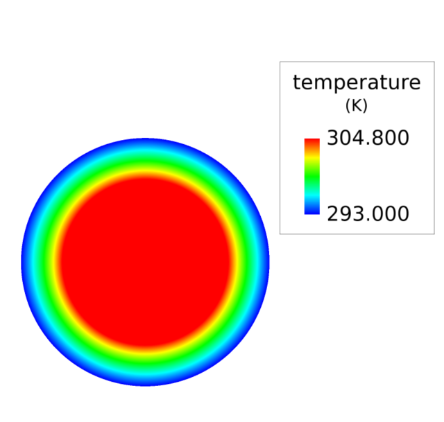
Figure 36.
Create an XY Plot for Temperature vs Radius
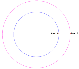
Figure 37.
-
From the Visualization toolbar, click the Plot icon
 .
The 2D Plot Controls and Plot Display dialogs open.
.
The 2D Plot Controls and Plot Display dialogs open. -
In the Edit Points dialog, enter the coordinate values for
the two points as shown below.
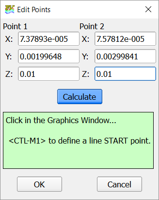
Figure 38. -
Click Calculate and OK to close
the dialog.
The Plot Display dialog is updated.
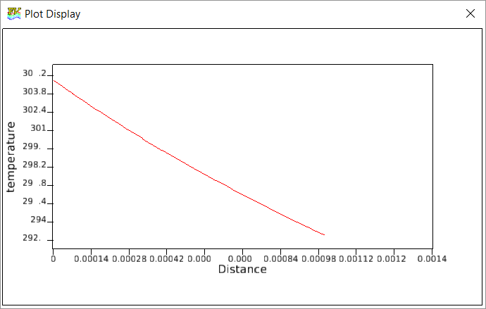
Figure 39. -
In the Horizontal Axis dialog:
- Change the Label to Radius (m).
- Change the Min value to 0.002.
- Change the Max value to 0.003.
- Change the Unit value next to Major to 0.0002.
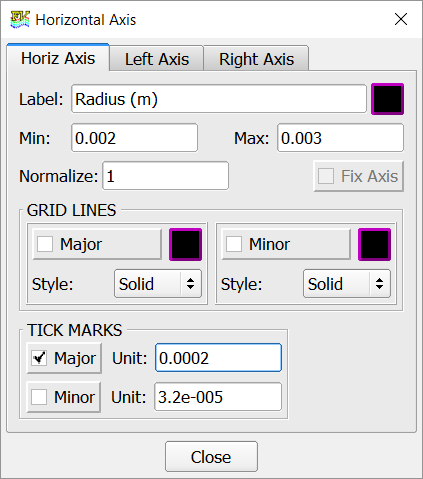
Figure 40. -
Change the Max value to 305 and the Unit value next to
Major to 2.
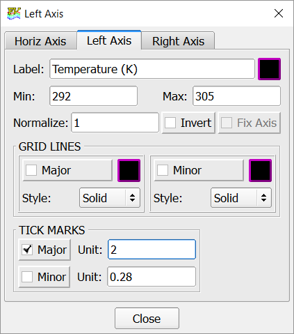
Figure 41. -
Click Close.
The Plot Display dialog is updated once more.
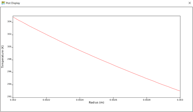
Figure 42.
Summary
In this tutorial, you worked through a basic workflow to set up a steady state simulation for a 2D cable problem. This problem was setup as a normal heat conduction problem where the inside solid volume was provided with a heat source. You started the tutorial by creating a database in AcuConsole, importing and meshing the geometry, and setting up the basic simulation parameters. Once the case was setup, the solution was generated with AcuSolve. Results were also post-processed in AcuFieldView by reading a dataset and viewing the temperature contours on the full geometry. New features that were introduced in this tutorial included the Electromagnetic Manager, which was used for importing a Nastran file that contained the thermal load applied to the SolidHeated volume, the variable manager, for defining all the variables in a single panel, mesh extrusion from one surface to the another surface along the length, reading a dataset in AcuFieldView, and finally, making 2D plots in AcuFieldView.