ACU-T: 3311 Multiphase Nucleate Boiling Using the Algebraic Eulerian Model
Prerequisites
This tutorial provides instructions for running a transient simulation of a two-phase Nucleate Boiling in a pipe using the Algebraic Eulerian model. Prior to starting this tutorial, you should have already run through the introductory HyperWorks tutorial, ACU-T: 1000 HyperWorks UI Introduction, and have a basic understanding of HyperMesh, AcuSolve, and HyperView. To run this simulation, you will need access to a licensed version of HyperMesh and AcuSolve.
Prior to running through this tutorial, copy HyperMesh_tutorial_inputs.zip from <Altair_installation_directory>\hwcfdsolvers\acusolve\win64\model_files\tutorials\AcuSolve to a local directory. Extract ACU-T3311_Steiner.hm from HyperMesh_tutorial_inputs.zip.
Since the HyperMesh database (.hm file) contains meshed geometry, this tutorial does not include steps related to geometry import and mesh generation.
Problem Description
The problem to be addressed in this tutorial is shown schematically in Figure 1. As an example, the Steiner problem is attached here to show the capability of the Multiphase Nucleate Boiling modeling in AcuSolve. The Algebraic Eulerian (AE) model with phase change is used to simulate the heat transfer and momentum exchange between a carrier field and a dispersed field.

Figure 1. Schematic of Channel
Open the HyperMesh Model Database
-
Click the Open Model icon
 located on the standard toolbar.
The Open Model dialog opens.
located on the standard toolbar.
The Open Model dialog opens.
Set the General Simulation Parameters
Set the Analysis Parameters
-
Set the Global Gravity in the Z direction to -9.8.
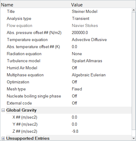
Figure 2.
Specify the Solver Settings
-
Verify that the Flow, Turbulence, and Field settings are turned
On.
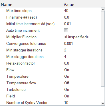
Figure 3.
Define the Nodal Outputs
-
Toggle on the Output initial condition field.
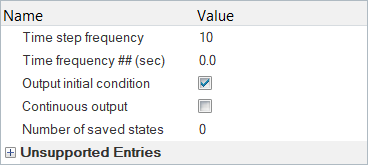
Figure 4.
Set Up Material Model Parameters
In this step, you will start by creating a new material named Vapor. Then, you will set up the Multiphase material model.
-
Set the Conductivity value to 0.02749.
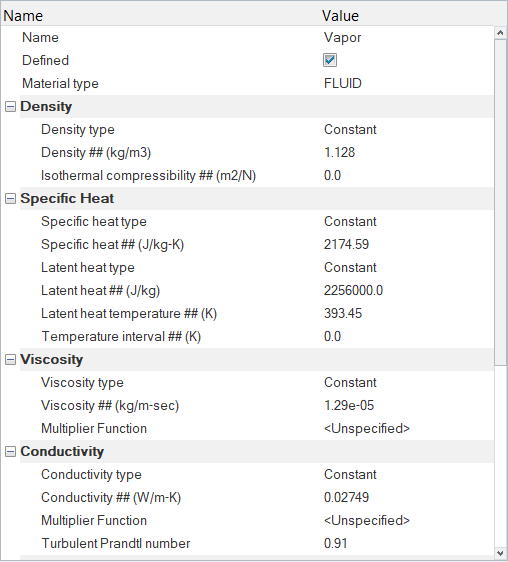
Figure 5. -
Verify that the Number of Dispersed Field is set to
1.
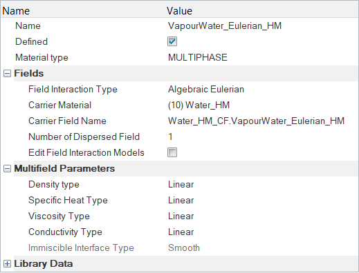
Figure 6. -
Set Dispersed field diameter type to Boiling Kurul
exponential.
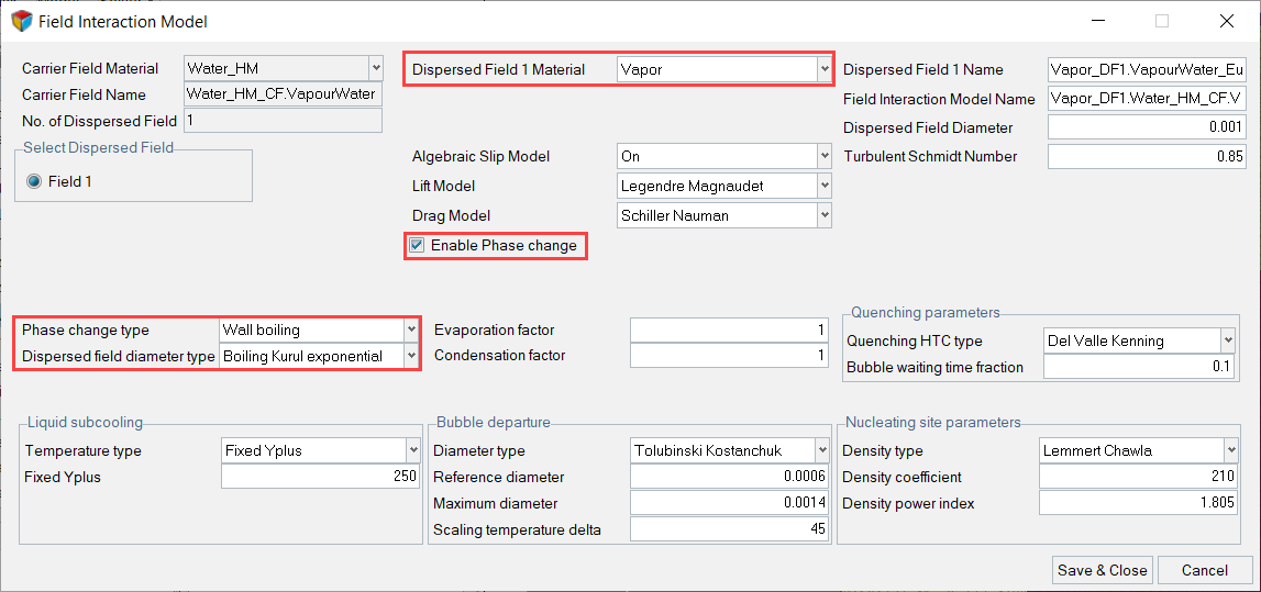
Figure 7.
Set Up Boundary Conditions and Nodal Initial Conditions
Set Up Boundary Conditions and Nodal Initial Conditions
In this step, you will assign the material properties to the multiphase fluid volume and then assign surface boundary conditions.
-
Click FluidVolume. In the Entity Editor,
- Change the Type to MULITPHASE if not set.
- Set VaperWater_Eulerian_HM as the Material.
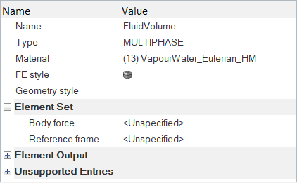
Figure 8. -
Click Inflow. In the Entity Editor,
-
Set the Temperature to 368.15.
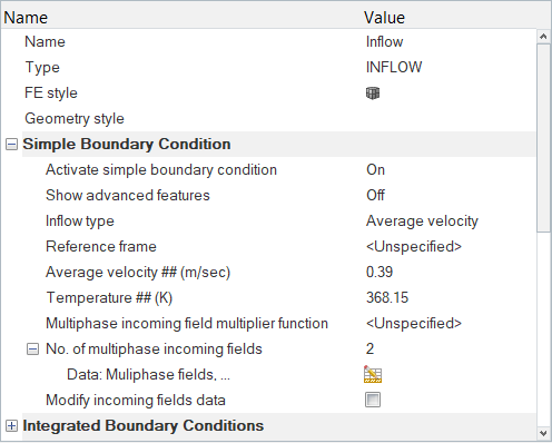
Figure 9. -
Similarly, select Vapor_DF1.
VaporWater_Eulerian_HM as the second Incoming Field and
set its Volume Fraction to 0.
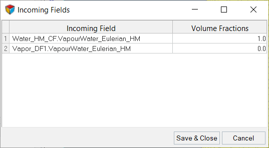
Figure 10.
-
Set the Temperature to 368.15.
-
Similarly, expand OUTFLOW then click the
Outflow component. In the Entity Editor, change the Type to
OUTFLOW if not set.
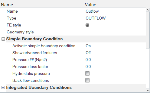
Figure 11. -
Similarly, expand WALL then click the
Side_MaxY component. In the Entity Editor, verify that the Type is set to
WALL.
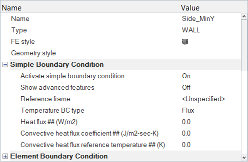
Figure 12. -
Click HeatedWall. In the Entity Editor,
- Verify that the Type is set to WALL.
- Set Temperature BC type to Value.
- Set the Temperature value to 403.15.
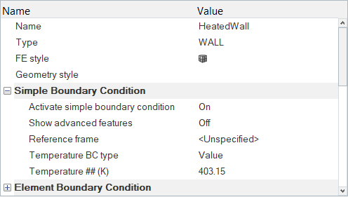
Figure 13.
Set the Nodal Initial Conditions
-
In the Fields dialog, set the values shown in the figure
below.
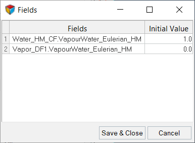
Figure 14.
Compute the Solution
In this step, you will launch AcuSolve directly from HyperMesh and compute the solution.
-
Click
 on the ACU toolbar.
The Solver job Launcher dialog opens.
on the ACU toolbar.
The Solver job Launcher dialog opens. -
Leave the remaining options as
default and click Launch to start the solution
process.
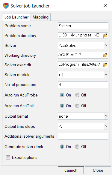
Figure 15.
Post-Process the Results with HyperView
Once the AcuSolve run is complete, close the HyperWorks Solver View dialog. In the HyperMesh Desktop window, close the AcuSolve Control and Solver job Launcher dialogs. In the next few steps, you will plot a contour of the vapor volume fraction.
Switch to the HyperView Interface and Load the AcuSolve Model and Results
-
In the HyperMesh Desktop window, click the
ClientSelector drop-down in the bottom-left corner of
the graphics window.
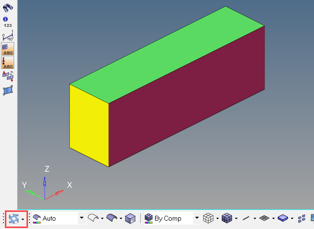
Figure 16. -
In the Load model and results panel, click
 next
to Load model.
next
to Load model.
Create Contours for the Volume Fraction of Vapor
-
Since this is a transient case, you need to plot the results at the last
timestep. To do this, click the Time drop-down menu in the Results Browser and select the last option in the list.
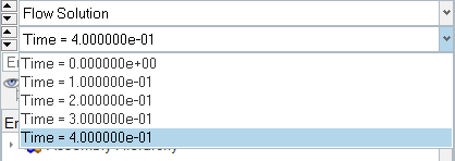
Figure 17. -
Click the Isolate Shown icon
 , hold Ctrl, then select the
HeatedWall and Bottom
components to turn off the display of all components except those that are
required.
, hold Ctrl, then select the
HeatedWall and Bottom
components to turn off the display of all components except those that are
required.
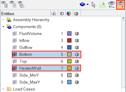
Figure 18. -
Click
 on the Results toolbar to open the Contour panel.
-
In the panel area, under the Display tab, turn off
the Discrete color option.
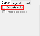
Figure 19. -
Click the Legend tab then
click Edit Legend. In the dialog, change the Numeric
format to Fixed then click
OK.
The contour plot should look similar to the figure below.
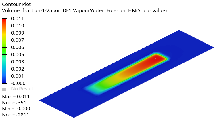
Figure 20.
Summary
In this tutorial, you worked through a basic workflow to set-up and solve a transient two-phase Nucleate Boiling flow problem using the Algebraic Eulerian multiphase model. You started by importing the model in HyperMesh. Then, you defined the simulation parameters and launched AcuSolve directly from within HyperMesh. Upon completion of solution by AcuSolve, you used HyperView to post-process the results and create a contour plot of the volume fraction.