ACU-T: 3101 Transient Conjugate Heat Transfer in a Mixing Elbow
This tutorial provides the instructions for setting up, solving and viewing results of 3D, turbulent flow with conjugate heat transfer in a mixing elbow. It is designed to introduce you to the AcuSolve tool set with a simple problem.
- Simulating transient flow characteristics
- Creating and applying multiplier functions
- Using the restart capability
- Decoupling of the flow and temperature simulations ("frozen" flow field for thermal simulations)
- Creating an animation from transient results
Prerequisites
You should have already run through the introductory tutorial, ACU-T: 2000 Turbulent Flow in a Mixing Elbow. It is assumed that you have some familiarity with AcuConsole, AcuSolve, and AcuFieldView. You will also need access to a licensed version of AcuSolve.
Prior to running through this tutorial, copy AcuConsole_tutorial_inputs.zip from <Altair_installation_directory>\hwcfdsolvers\acusolve\win64\model_files\tutorials\AcuSolve to a local directory. Extract MixingElbow_ColdSlug.acs from AcuConsole_tutorial_inputs.zip.
Analyze the Problem
An important first step in any CFD simulation is to examine the engineering problem to be analyzed and determine the settings that need to be provided to AcuSolve. Settings can be based on geometrical components (such as volumes, inlets, outlets, or walls) and on flow conditions (such as fluid properties, velocity, or whether the flow should be modeled as turbulent or as laminar).
The problem is divided into two components, a steady state solution and a transient solution. The flow and thermal fields that are established in the steady simulation will be used as a starting point for the transient simulation. The use of these "frozen" flow and thermal fields dramatically reduces the overall solution time necessary to solve the thermal transient model. This technique of solving temperature separate from the flow field is a powerful feature that can be applied to a broad class of problems. Note that this simulation approach relies on decoupling of the thermal and momentum fields. If there is strong coupling between the flow and thermal fields (that is, through temperature-dependent material properties), this approach cannot be applied.
Analyze the Steady State Component
The steady state portion of the problem is shown schematically in Figure 1. It consists of a mixing elbow made of stainless steel with water entering through two inlets with different velocities and with different temperatures.
This case is the same as the one used in ACU-T: 3100 Conjugate Heat Transfer in a Mixing Elbow. The geometry is symmetric about the XY midplane of the pipe, as shown in the figure. This symmetry allows the flow to be modeled with the use of a symmetry plane. The use of a symmetry plane leads to reduced computation time while still providing an accurate solution.

Figure 1. Schematic of Mixing Elbow with Stainless Steel Walls
Details of the problem characteristics are shown in the following images extracted from a sample worksheet that was created prior to setting up the case for AcuSolve.
The diameter of the large inlet is 0.1 m, the inlet velocity (v) is 0.4 m/s and the temperature (T) of the fluid entering the large inlet is 295 K. The diameter of the small inlet is .025 m, the velocity is 1.2 m/s, and the temperature of the fluid entering the small inlet is 320 K. The pipe wall has a thickness of 0.005 m.
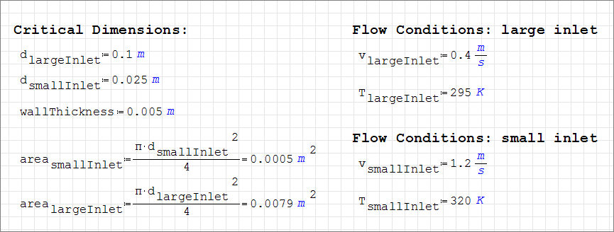
Figure 2.
The fluid in this problem is water, with the following properties that do not change with temperature; a density (ρ) of 1000 kg/m3, a molecular viscosity (μ) of 1 X 10⁻³ kg/m-sec, a conductivity (k) of 0.598 W/m-K, and a specific heat (cp) of 4183 J/kg-K, as shown in the worksheet.
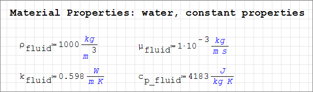
Figure 3.
The pipe walls are made of stainless steel with a density of 8030 kg/m3, a conductivity of 16.2 W/m-K, and a specific heat of 500 J/kg-K.
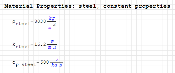
Figure 4.
Based on mass conservation, the combined flow rate (Q) yields a velocity of 0.475 m/s downstream of the small inlet. This value is useful in determining the Reynolds number, which in turn can be used to determine if the flow should be modeled as turbulent, or if it should be modeled as laminar.
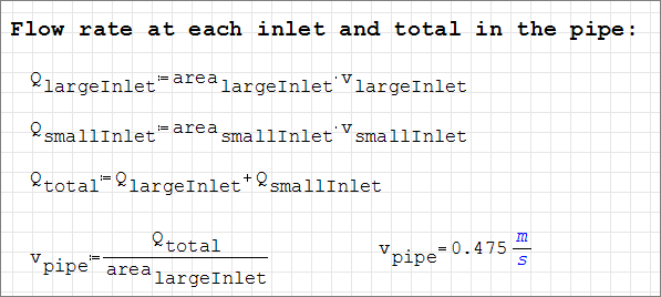
Figure 5.
The Reynolds numbers of 40,000 at the large inlet, 30,000 at the small inlet, and 47,500 for the combined flow indicate that the flow is turbulent throughout the flow domain.
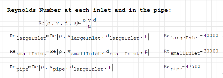
Figure 6.
The simulation will be set up to model steady state, turbulent flow. In addition, the thermal characteristics of the flow will be modeled using advection and diffusion equations.
The simulation will be set up to model steady state, turbulent flow. In addition, the thermal characteristics of the flow will be modeled using advection and diffusion equations. The simulation will be set up to model steady state, turbulent flow with varying temperature.
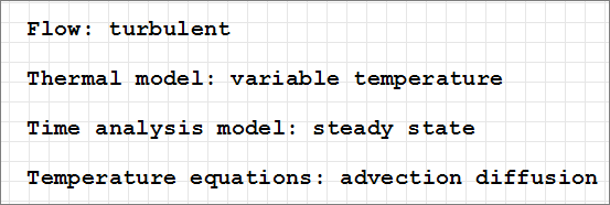 Figure 7.
 In addition to setting appropriate conditions to capture the physics of the simulation, it is important to generate a mesh that is sufficiently refined to provide good results. In this tutorial the global mesh size is set to provide at least 30 mesh elements around the circumference of the large inlet. For this problem, the global mesh size is 0.0106 m. This mesh size was chosen to provide a quick turnaround time for the model. For real-world simulations, you would modify your mesh settings after an initial solution until a mesh-independent solution is reached (that is, a solution that does not change with further mesh refinement).
AcuSolve allows for mesh refinements in a user-defined region that is independent of geometric components of the problem such as volumes, model surfaces, or edges. It is useful to refine the mesh in areas where gradients in pressure, velocity, eddy viscosity, and the like are steep. For this problem , the flow entering the large pipe from the side pipe creates large velocity gradients that need to be resolved. A mesh refinement zone is used to capture the flow in this region.
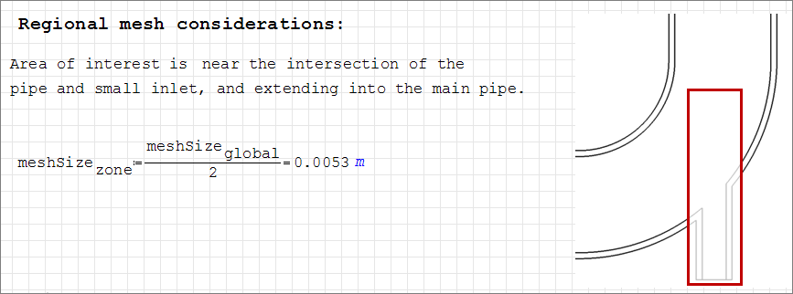
Figure 8.
Once a steady state solution is calculated, you will create a transient database, modify settings, and solve for the transient temperature characteristics of the problem.
Analyze the Transient Component
The starting point for the transient portion of the problem is shown schematically in Figure 9. It consists of a mixing elbow with a steady state solution for flow and temperature. A cold slug of water is injected at both inlets during the simulation. The temperature excursion drops the temperature at both inlets to 283.15 K for a duration of 1.0 s.
Figure 9. Schematic of Initial Conditions of Mixing Elbow
The temperature profile at the inlets is shown in Figure 10. The temperature of the water flowing in the large inlet at t=0 is 295 K and the temperature of the fluid flowing in the small inlet at t=0 is 320 K. The temperature is held constant for 0.2 s, then is ramped down at both inlets and reaches 283.15 K at 0.4 s into the simulation. The temperature is held constant for 1 s. The temperature is ramped up beginning at 1.4 s, and by 1.6 s the inlet temperatures are back to their initial states.
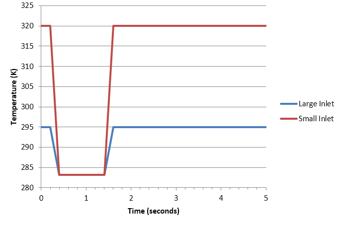
Figure 10. Transient Temperature Profile at Inlets
For this case, the minimum duration would be the time it takes for the cold slug to move completely through the domain. This minimum period is given by the steady state transit time through the domain added to the duration of the cold slug.
Transit time can be estimated using the inlet velocity at the large inlet and the estimated length of the flow path. The flow path is made up of a straight section 0.2 m long (l1), a 90-degree elbow section with an average radius of 0.15 m (lelbow), and another straight section 0.2 m long (l2).
Figure 11.
The inlet velocity for the large inlet is 0.4 m/s. Given a flow path of 0.6356 m, the transit time will be approximately 1.6 s. In order to predict the movement of the cold slug through the domain, our simulation period would be at least 3.2 s.
Figure 12.
To allow time for the thermal conditions to return to the steady state, additional time can be added to the simulation. For this case 1.3 s will be added for a total simulation period of 4.5 s.
Figure 13.
Another critical decision in a transient simulation is choosing the time increment. The time increment is the change in time during a given time step of the simulation. It is important to choose a time increment that is short enough to capture the changes in flow properties of interest, but does not require unnecessary computation time.
There are two methods commonly used for determining an appropriate time increment. The first method involves identification of the time scales of the transient behaviors of interest and setting the time increment to sufficiently resolve those behaviors. The second method involves setting a limit on the number of mesh elements that the flow can cross in a given time step. A convenient metric for the number of mesh elements crossed per time step is the Courant-Friederichs-Lewy number, or CFL number. With this method, the time increment can be computed from the mesh size, the flow velocity, and the desired CFL number. In this tutorial, the time increment was calculated using the global mesh size and a CFL number of 2, ensuring that any portion of the cold slug will not advance past more than 2 mesh elements within a given step. For a real-world problem, you would base your calculations on the mesh size at in the mesh zone of interest.
Figure 14.
The temperature change at the large inlet is from 295 K to 283.15 K. At the small inlet the temperature changes from 320 K to 283.15 K. The ratio of the cold slug temperature to the initial temperature of the large inlet flow is 0.9598. The ratio of the cold slug temperature to the initial temperature of the small inlet flow is 0.8848. These values will be used in creating multiplier functions to model the transient temperatures at the inlets.
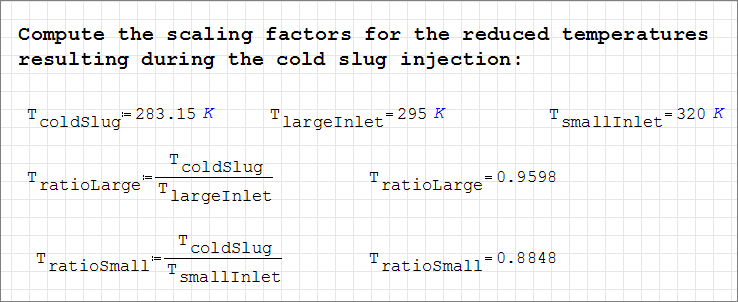
Figure 15.
Once a transient solution is calculated, the results of interest are the transient thermal characteristics of the fluid and pipe walls at different times in the simulation.
Define the Simulation Parameters
Start AcuConsole and Solve the Steady State Simulation
In the next steps you will start AcuConsole and open a database that is set up for a steady state simulation for flow and conjugate heat transfer. You will then run AcuSolve to calculate a steady state solution, view the results with AcuFieldView, and save the database for the transient simulation.
- Start AcuConsole from the Windows Start menu by clicking .
-
Open MixingElbow_ColdSlug.acs.
- Click .
- Browse to the directory containing Mixing_Elbow_Cold_Slug\Completed-Steady.
- Select MixingElbow_ColdSlug.acs and click Open to open the database.
-
Run AcuSolve to solve the steady state problem.
-
Click
 on the toolbar to open the
Launch AcuSolve dialog.
on the toolbar to open the
Launch AcuSolve dialog.
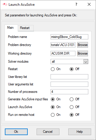
Figure 16.Based on these settings, AcuConsole will generate the AcuSolve input files, then launch the solver. AcuSolve will run on four processors to calculate the steady state solution for this problem.
-
Click Ok to start the
solution process.
During meshing an AcuTail window opens. Meshing progress is reported in this window. A summary of the meshing process indicates that the mesh has been generated.
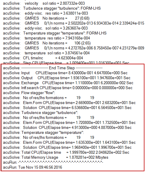
Figure 17.
-
Click
Steady State Results
The steady state flow field was calculated as the starting point for the transient simulation of temperature. For instructions on visualising steady state results, refer to ACU-T: 3100 Conjugate Heat Transfer in a Mixing Elbow.
Create the Transient Simulation Database
The transient portion of the simulation will use the same geometry and many of the same attributes as used in the steady state simulation. As such, you can create a copy of the steady state database and then modify the settings as needed to set up the transient simulation. You will save the transient database in a different directory to avoid confusion of the steady and transient runs.
In these steps you will create the transient database.
- Click .
- Browse up one level to the ..\Mixing_Elbow_Cold_Slug directory.
- Enter mixingElbow_ColdSlug as the File name.
- Click Save.
Set General Simulation Parameters
In the next steps you will modify global settings needed for the transient portion of the simulation.
The general attributes that you will modify for the transient simulation are the subtitle and the analysis type.
-
Click BAS in the Data Tree Manager to switch to basic view in the Data Tree.
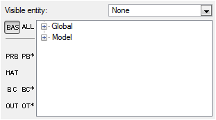
Figure 18. -
Double-click the Global
Data Tree item to expand it.
Tip: You can also expand a tree item by clicking
 next to the item name.
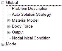
Figure 19. -
Change the Analysis type to Transient.
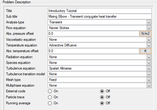
Figure 20.
Set Solution Strategy Parameters
In the next steps you will set attributes that control the behavior of AcuSolve as it progresses during the transient solution.
Figure 21.
-
Click Off next to Turbulence to turn off the solving of
the turbulence equation.
By turning these options off, AcuSolve will not update the solution to these equations. Instead, the current flow and turbulence values (generated from the steady state solution for this tutorial) will be used throughout the simulation and AcuSolve will only solve for the temperature field.
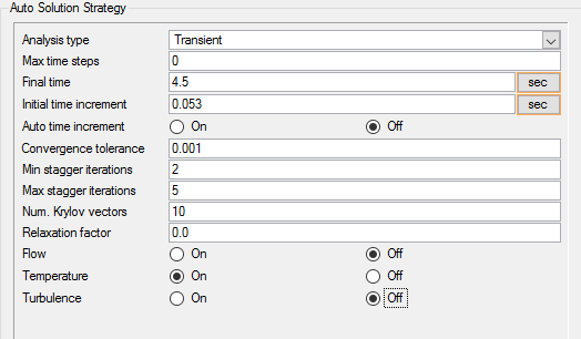
Figure 22.
Set Nodal Output Frequency
In the next steps you will set an attribute that impacts how often results from the transient simulation are written to disk. Writing the results every three time steps produces a collection of output states that can be used to create an animation of the simulation once the run has completed. Note that more frequent output can be used, but it will result in higher disk space usage.
-
Enter 3 as the Time step frequency.
This value indicates that AcuSolve should write results after every three time steps.
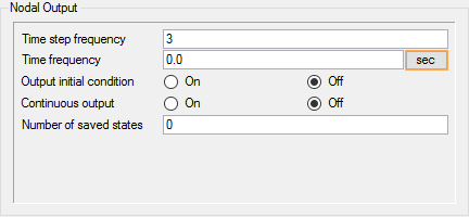
Figure 23.
Create Multiplier Functions for Transient Inlet Temperatures
AcuSolve provides the ability to scale values as a function of time and/or time step during a simulation. This is achieved through the use of a multiplier function. In this tutorial, the inlet temperature varies as the simulation progresses. By taking advantage of multiplier functions, you can easily set up functions to model the temperature changes at the inlets.
In the next steps you will create a multiplier function for the temperature at the large inlet, duplicate it, and modify the copy to be used with the small inlet. These multiplier functions will be applied to the large and small inlets later in this tutorial.
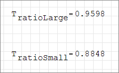
Figure 24.
In this tutorial, the inlet temperatures drop from initial conditions to 283.15 K, are held at that temperature, and then ramp back up to the initial temperatures.
Figure 25.
To make the creation of the multiplier functions as simple as possible, you will use the PB* filter in the Data Tree Manager.
-
Click PB* in the Data Tree Manager
to show all problem-definition settings.
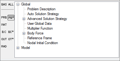
Figure 26. -
Set the Type to Piecewise Linear.
This option indicates that you will enter an array of numbers that will be used by AcuSolve to interpolate the value of the multiplier function at each time step. In this example, the curve fit is a function of time.
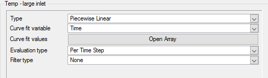
Figure 27. -
Add the curve-fit values for the large inlet temperature profile.
-
Repeat this process until you have entered all of the values shown in
the figure below.
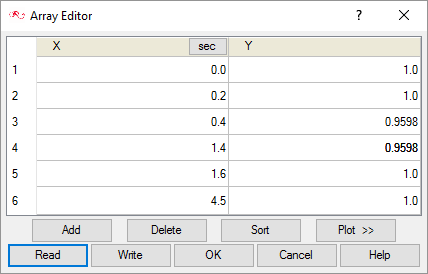
Figure 28. -
Click Plot to expand the
Array Editor dialog to display the plot of the
curve fit values.
You may need to expand the dialog by dragging the right edge in order to see the plot.
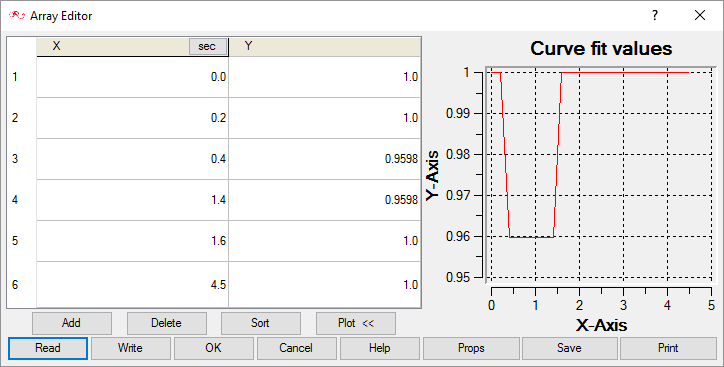
Figure 29.
-
Repeat this process until you have entered all of the values shown in
the figure below.
Define Transient Inlet Boundary Conditions
In the following steps you will set the inlet boundary conditions that produce the time varying temperatures at the large and small inlets. This will be achieved by modifying the boundary conditions to use the multiplier functions that you created earlier in this tutorial.
Set Transient Temperature for the Large Inlet
In the next steps you will associate the Temp - large inlet multiplier function with the large inlet boundary condition.
-
Change Temperature multiplier function to Temp - large
inlet.
This instructs AcuSolve to determine the inlet boundary value for temperature by first evaluating the multiplier function, then multiplying its value by the specified value of temperature. Since the multiplier-function value changes as a function of time, the inlet temperature will change as a function of time.
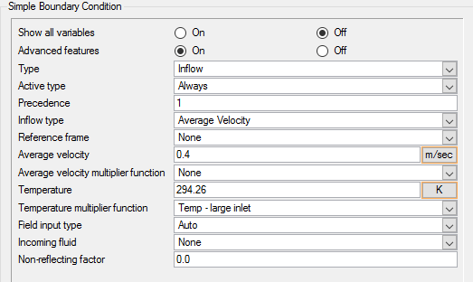
Figure 30.
Set Transient Temperature for the Small Inlet
In the next steps you will associate the Temp - small inlet multiplier function with the small inlet boundary condition.
-
Change Temperature multiplier function to Temp - small
inlet.
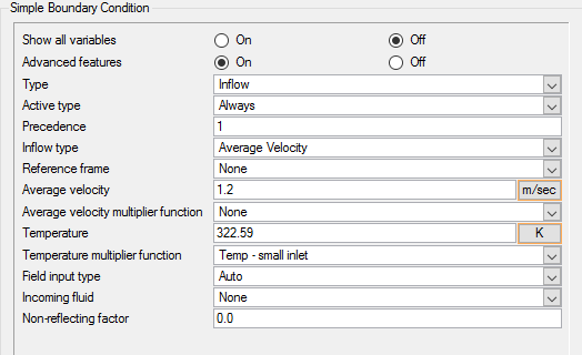
Figure 31.
Compute the Solution and Review the Results
Run AcuSolve
In the next steps you will modify the AcuSolve settings to run the transient solution. The main feature that you will use is a restart. A restart allows you to start a solution based on the results of a previous solution. In this case, the flow and thermal field from the initial solution that you performed in this tutorial will be used as the starting point. Since the flow and turbulence equations were turned off when defining the solution strategy, the temperature field is the only one that will be solved.
-
Click
 on
the toolbar to open the Launch AcuSolve dialog.
on
the toolbar to open the Launch AcuSolve dialog.
-
Verify that the following restart options are set appropriately:
Note: You can drag the right edge of the dialog to make it wider.
From run 0 From time step 0 Reset time step On Reset time increment On 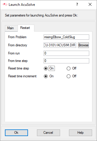
Figure 32. -
Click Ok to start the
solution process.
While computing the solution, an AcuTail window opens. Solution progress is reported in this window. A summary of the solution process indicates that the run has been completed.
The information provided in the summary is based on the number of processors used by AcuSolve. If you use a different number of processors than indicated in this tutorial, the summary for your run may be slightly different than the summary shown.
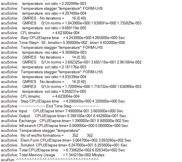
Figure 33.
View Transient Results with AcuFieldView
Now that transient results have been calculated, you are ready to review the flow field with AcuFieldView. AcuFieldView is a third-party post-processing tool that is tightly integrated to AcuSolve. AcuFieldView can be started directly from AcuConsole, or it can be started from the Start menu, or from a command line. In this tutorial you will start AcuFieldView from AcuConsole after the solution is calculated by AcuSolve.
In the following steps you will display the temperature contours for the fluid and for the pipe walls on the symmetry plane, add velocity vectors to the view, then animate the results.
Start AcuFieldView
-
Click
 on the
AcuConsole toolbar to open the
Launch AcuFieldView dialog.
on the
AcuConsole toolbar to open the
Launch AcuFieldView dialog.
Display Contours of Fluid and Solid Temperature on the Symmetry Plane
In the next steps you will create a boundary surface to display contours of fluid and solid temperature on the symmetry plane at the end, middle, and beginning of the transient simulation. The first visualization will be for the last time step in the simulation, which is the last set of results loaded from AcuSolve when AcuFieldView was started.
-
Click
 to open the Boundary
Surface dialog.
Note: The dialog may already be open. This step will put the focus on the dialog.
to open the Boundary
Surface dialog.
Note: The dialog may already be open. This step will put the focus on the dialog. -
On the toolbar, click the Colormap icon
 .
.
-
Set the colormap to cover the range of temperatures
used in the simulation.
- In the Boundary Surface dialog, click the Colormap tab.
- Enter 323 as the upper value for Scalar Coloring.
- Enter 282 as the lower value for Scalar Coloring.

Figure 34. -
Add a legend to the view.
- Click the Legend tab in the Boundary Surface dialog.
- Enable the Show Legend option.
- Enable the Frame option.
- Click the white color swatch next to Geometric in the Color group and set the color for the legend values to black.
- Set Decimal Places to 1.
- Click the white color swatch next to the Title field and set the color for the title to black.
- Enter transient as the Subtitle.
- Click the white color swatch next to the Subtitle field and set the color to black.
- Move the legend by Shift+left-clicking and dragging the legend to the left.

Figure 35.This image was created with a white background, perspective turned off, outlines turned off, and the viewing direction set to +Z.
When AcuFieldView is run from a transient AcuSolve case, the results from the final time step are shown by default.
-
Display contours of temperature at the middle of the transient
simulation.
-
Click the Tools menu
and then click Transient Data to open the
Transient Data Controls dialog.

Figure 36.Note: Note that the slider under Solution Time is all the way to the right. The contours currently displayed are from the end of the simulation.
-
Move the slider control to Time Step 42, or enter
42 in the field, and click
Apply.
The resulting contours show the thermal conditions at time step 42.
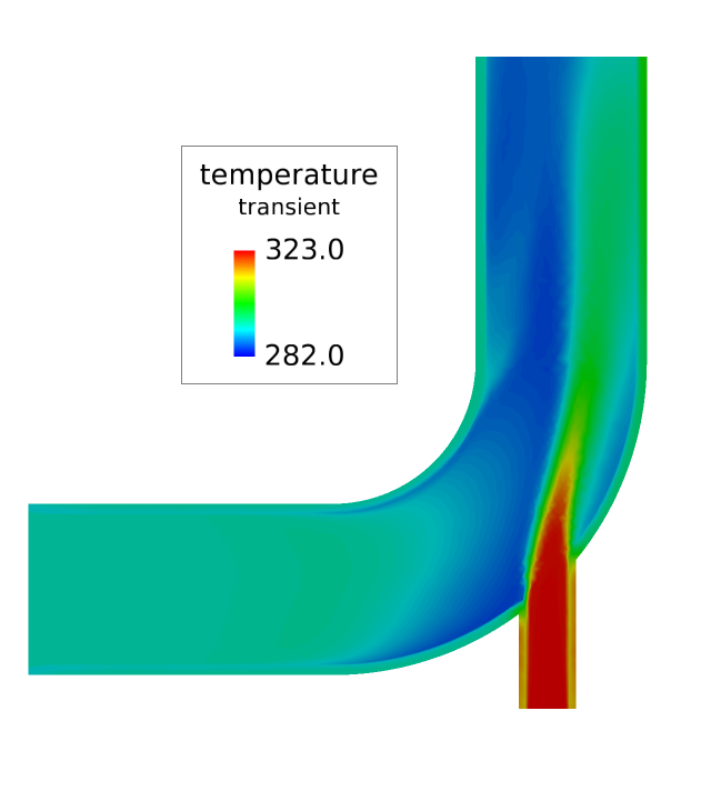
Figure 37.
-
Click the Tools menu
and then click Transient Data to open the
Transient Data Controls dialog.
-
Display contours of temperature at the start of the transient simulation.
-
Move the slider control to the beginning of the range and click
Apply.
The resulting contours show the thermal conditions for a time step at the beginning of the simulation.
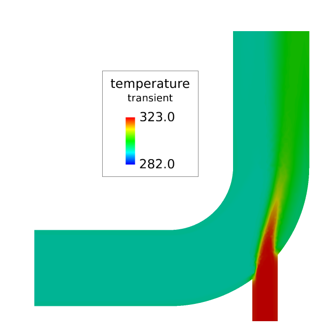
Figure 38.
Note that the contours from the beginning of the simulation are similar to those from the end of the simulation. The conditions changed as the cold slug propagated through the pipe, and then returned to initial conditions. The contours from the middle of the simulation show that the steel-wall temperature near the intersection of the small pipe was higher than for the nearby water, reflecting a lag in the temperature change of the wall compared to the water. -
Move the slider control to the beginning of the range and click
Apply.
Add Velocity Vectors to the View
In the next steps you will create a new boundary surface and display velocity vectors on that surface.
The resulting visualization will be compared to the one created for the steady state solution.
-
Set vector options.
-
Click Options next to
Vectors to open the Vector Options dialog.
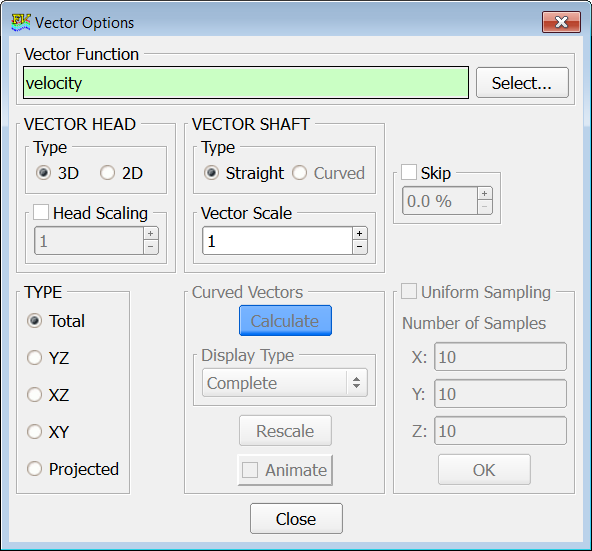
Figure 39.
-
Click Options next to
Vectors to open the Vector Options dialog.
-
Set the symmetry plane as the location for
display of the vectors.
- Click OSF: Symmetry in the list of Boundary Types.
- Click OK.
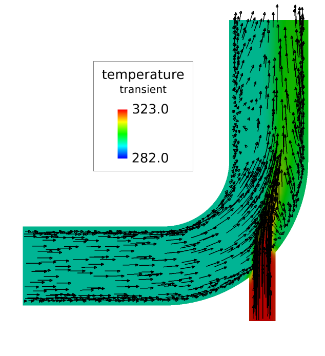
Figure 40.
Display Transient Temperature Contours
In the next steps you will view the transient thermal data for the cold slug.
-
Click the Tools menu and then
click Transient Data to open the Transient Data
Controls dialog.
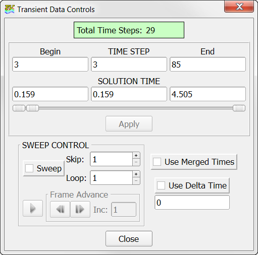
Figure 41. -
Change the playback rate.
-
Click the View menu and then click
Minimum Time Between Frames.

Figure 42.
With the Sweep Control options, pause the sweep, advance or reverse frames, and play the sweep. -
Click the View menu and then click
Minimum Time Between Frames.
Animate the Transient Temperature Sweep
In the next steps you will create a transient sweep and save it as an animation that can be viewed independently of AcuFieldView.
-
Click OK to dismiss
the Flipbook Size Warning dialog.
The Sweep button on the Transient Data Controls dialog will have changed to Build.
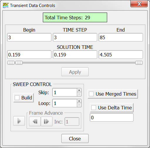
Figure 43. -
Click Build.
As AcuFieldView builds the flipbook animation, you will see the controls on the Transient Data Controls dialog advance. Once the flipbook is built, a Flipbook Controls dialog will allow you to play or save the animation.
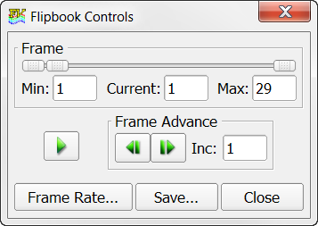
Figure 44. -
Click
 to play the animation.
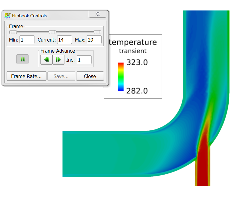
Figure 45. -
Click
 to pause the playback.
Summary
In this tutorial, you worked through a basic workflow to set up a transient simulation case. You were provided with a fully set up steady state case to use as initial conditions for the transient simulation. The transient simulation was carried out using the "frozen flow" methodology to simulate the transient temperature field without recomputing the velocity field. Once the transient case was set up and solved, results were post-processed in AcuFieldView to allow you to create contour and vector views along the symmetry plane of the model, and to animate the temperature contours. New features introduced in this tutorial include transient simulation, multiplier functions, restarts, frozen flow and animation of transient results.