ACU-T: 3000 Enclosed Hot
Cylinder: Natural Convection
This tutorial provides the instructions for setting up, solving and viewing
results for a simulation of a hot cylinder contained within another
air-filled cylinder. In this simulation, an internally heated cylinder is
surrounded by air which heats up as it comes in contact with the surface of
the inner cylinder. The localized heating near the surface induces a
buoyancy driven flow in the air, generating convection currents. This
tutorial is designed to introduce you to modeling concepts related to
natural convection simulations.
The basic steps in any CFD simulation are shown in ACU-T: 2000 Turbulent Flow in a Mixing Elbow. The following additional
capabilities of AcuSolve are introduced in this
tutorial:
Creating and specifying a new custom material in AcuConsole
Specifying a volume group as a heat source
Using the Boussinesq density model in buoyancy driven flows,
such as cases involving natural convection
Set up periodic boundary conditions
In this tutorial you will do the following:
Analyze the problem
Start AcuConsole and create a
simulation database
Set general problem parameters
Set solution strategy parameters
Create a new custom material model in AcuConsole and assign material
properties to it
Import the geometry for the simulation
Create a volume group and apply volume parameters
Create surface groups and apply surface parameters
Set global and local meshing parameters
Set periodic boundary conditions
Generate the mesh
Set the appropriate boundary conditions
Run AcuSolve
Monitor the solution with AcuProbe
Post-processing the nodal output with AcuFieldView
Prerequisites
You should have already run through the introductory tutorial, ACU-T: 2000 Turbulent Flow in a Mixing Elbow. It is assumed that you have some
familiarity with AcuConsole, AcuSolve, and AcuFieldView. You will
also need access to a licensed version of AcuSolve.
Prior to running through this tutorial, copy
AcuConsole_tutorial_inputs.zip from
<Altair_installation_directory>\hwcfdsolvers\acusolve\win64\model_files\tutorials\AcuSolve
to a local directory. Extracttwin_cylinder.x_tfrom AcuConsole_tutorial_inputs.zip.
The color of objects shown in the modeling window in this tutorial and those displayed on your screen may differ. The default color
scheme in AcuConsole is "random," in which colors are
randomly assigned to groups as they are created. In addition, this tutorial was
developed on Windows. If you are running this tutorial on a different operating system,
you may notice a slight difference between the images displayed on your screen and the
images shown in the tutorial.
Analyze the Problem
An important step in any CFD simulation is to examine the engineering problem at hand and
determine the important parameters that need to be provided to AcuSolve. Parameters can be based on geometrical elements (such as inlets, outlets, or walls) and on
flow conditions (such as fluid properties, velocity, or whether the flow should be modeled as
turbulent or as laminar).
The system being simulated contains an internally-heated cylinder, which is surrounded by a
cylindrical ring of a larger diameter. The annular volume between the two cylinders is filled
with a fluid (air). The inner cylinder thus acts a heat source, and the fluid in contact with the
surface of this heat source is heated up. This hot fluid, being lower in density than the cold
fluid, then rises up to the upper part of the annulus due to buoyancy effects, and displaces the
cold fluid at top. At the same time, the film of fluid which was in contact with the heating
surface is replaced by the surrounding cold fluid. This new film of cold fluid goes through the
same process until eventually a steady state convection current is achieved, or the inner
cylinder ceases to generate heat and slowly the whole system achieves an equal temperature.
The system being simulated can be considered similar to a heat exchanger wherein the inner
cylinder is akin to a tube through which a hot fluid passes by, and the air which surrounds this
inner tube extracts heat from the inner tube. Another analogy can be of a wire carrying high
current enclosed in an air cooled chamber. As the current heats up the wire due to resistance,
the air around the wire keeps the wire temperature within control by extracting heat from the
wire surface.
The schematics of the problem which will be addressed in this tutorial is shown in Figure 1. The inner cylinder is a solid
volume with internal heat generation, and the outer cylinder is a fluid volume with air as the
fluid. Both cylinders are assumed to be infinitely long and the system will be modeled using half
symmetry and periodicity. The cylinders are infinite in z-direction and hence periodicity will be
applied along this direction. Figure 1. Schematic of the Problem
Introduction to Theory
Natural Convection
Convection is a heat transfer mechanism where the transfer of heat energy happens through the
motion of matter. Since the definition of convection involves motion of matter a fluid state is
usually present in convection. Usually this type of heat transfer takes place between a hot or a
cold surface and a fluid. The film of fluid in contact with the surface absorbs heat from or
transfers heat to the surface and is then replaced by a new film. This movement of fluid may
either be governed by an external source, such as a fan or pump, or due to internal changes in
the fluid properties. When no external sources are responsible for the fluid motion the heat
transfer mechanism at work is called the Natural Convection. The driving force for motion of the
fluid in a natural convection is density changes in the fluid due to temperature gradients
induced in the fluid by heat transfer.
The natural convection mechanism works similarly as described above, whilst discussion of the
problem. The fluid which is in contact with the surface absorbs or transfers heat from the
surface and becomes hotter or colder than the surrounding fluid. Driven by buoyancy forces due to
difference in densities caused by the temperature gradient, the fluid is displaced upwards or
downwards. Surrounding fluid fills in the void created by the displaced fluid, which then
undergoes the same process again. This gives rise to a convection current which drives the hot
fluid to the top and cold fluid to the bottom of the convection cell. Buoyancy effects are driven
by gravity, therefore natural convection requires presence of a gravitational force to work. It
must be noted, however, that gravity is not the driving force behind the fluid movement. Presence
of gravity only enables displacement of the fluid due to the density changes caused by
temperature gradients.
Mathematical determination of the onset of natural convection is done through a dimensionless
number called the Rayleigh number (Ra). The Rayleigh number is defined as:
where:
x is the characteristic length (m)
is the Rayleigh number for characteristic length x
is acceleration due to gravity (m/s2)
is the surface temperature (K)
is the quiescent temperature (fluid temperature far from the surface of the object)
(K)
is the kinematic viscosity (m2/s)
α is the thermal diffusivity (m2/s)
β is the thermal expansion coefficient (equals to for ideal gases where is absolute temperature).
The fluid properties , α and β are evaluated at the film temperature, , which is defined as:
When the Rayleigh number is below a critical value for the fluid heat transfer is primarily in
the form of conduction. When it exceeds this critical value the dominant heat transfer mechanism
is convection.
Boussinesq Density Model
The Boussinesq density model is an approximation method applied to buoyancy driven flows, such
as natural convection flows. In the Boussinesq approximation, the density variation terms are
neglected everywhere except when multiplied by acceleration due to gravity, . The basis of this approximation is that since temperature changes are small, the
resultant changes in density are small as well and thus can be neglected. However, when
multiplied by , the resultant term gives rise to forces which no longer are negligible. The Boussinesq
approximation is:
where
is the instantaneous density at temperature (kg/m3)
is the density at reference temperature (kg/m3)
is change in temperature (K)
As stated in the approximation, the Boussinesq density model is only applicable when density
variations are small. A general guideline is to check for the condition to be true. This indirectly puts a limitation on this model to be used to only for
cases where expected temperature differences within the fluid are not large.
Define the Simulation Parameters
Start AcuConsole and Create the Simulation Database
In this tutorial, you will begin by creating a database, populating the
geometry-independent settings, loading the geometry, creating volume and surface
groups, setting group parameters, adding geometry components to groups, and
assigning mesh controls and boundary conditions to the groups. Next, you will
generate a mesh and run AcuSolve to solve for the number
of time steps specified. Finally, you will visualize some characteristics of the
results using AcuFieldView.
In the next steps you will start AcuConsole, and create
the database for storage of the simulation settings.
Start AcuConsole from the Windows Start menu by clicking Start > Altair <version> > AcuConsole.
Click the File menu, then click
New to open the New data
base dialog.
Note:You can also open the
New data base dialog by clicking on the toolbar.
Browse to the location that you would like to use as your working
directory.
This directory is where all files related to the simulation will
be stored. The AcuConsole database file
(.acs) is stored in
this directory. Once the mesh and solution are created, additional files and
directories will be created within this directory.
Create a new directory in this location. Name it
Natural_convection and navigate into this
directory.
Enter NaturalConvection as the file name for the
database, or choose any name of your preference.
Note: In order for other applications to be able to read the
files written by AcuConsole, the database
path and name should not include spaces.
Click Save to create the database.
Set General Simulation Parameters
In next steps you will set parameters that apply globally to
the simulation. To make this simple, the basic settings applicable for any
simulation can be filtered using the BAS filter in the Data Tree Manager. This filter enables display of only a small subset
of the available items in the data tree and makes navigation of the entries
easier.
Click BAS in the Data Tree Manager to switch to basic view in the Data Tree.
Figure 2.
Double-click the GlobalData Tree item to expand it.
Tip: You can also expand a tree item
by clicking
next to the item name. Figure 3.
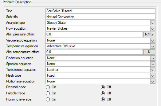
Double-click Problem
Description to open the Problem
Description detail panel.
Tip: You can also open a panel by right-clicking a tree item and
clicking Open on the context menu.
Enter AcuSolve Tutorial as the Title.
Enter Natural Convection as the Sub title.
Change the Analysis type to Steady State.
Change the Temperature equation to Advective
Diffusive.
Figure 4.
Set Solution Strategy Parameters
In the next steps you will set the parameters that control
the behavior of AcuSolve as it progresses during the
solution.
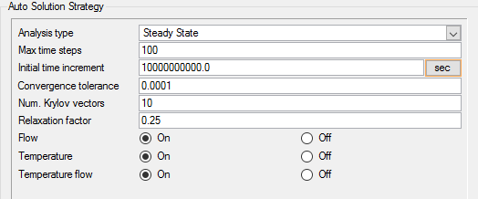
Double-click Auto Solution
Strategy in the Data Tree to open the
Auto Solution Strategy detail panel.
Check that Analysis type is set to Steady State.
Set the Max time steps to 100.
Change the Convergence tolerance to 0.0001.
Enter 0.25 for the Relaxation
factor.
Check that Flow and Temperature are set to On.
Change the Temperature flow to On.
Changing the Temperature flow flag to On will instruct the solver to solve
thermal-flow problems in fully coupled mode. Otherwise these problems are solved
with a staggered strategy. In fully-coupled mode, the flow and temperature
equations are solved simultaneously, while in the staggered approach, the flow
equation will usually be solved first considering constant temperature, and then
the temperature equation will be solved as the next step. Figure 5.
Set Material Model Parameters
AcuConsole has three pre-defined materials, Air,
Aluminum and Water, with standard parameters defined. In the next steps you will check
and modify the material characteristics of the predefined Air model to match the desired
properties for this problem. Since this a natural convection problem the density type
for air will be set to use the Boussinesq approximation. Subsequently, you will create a
new custom material and assign relevant material properties to it.
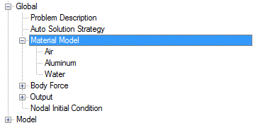
Double-click Material Model
in the Data Tree to expand it.
Figure 6.
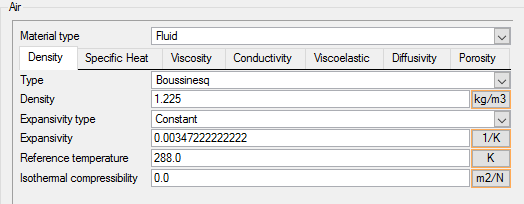
Double-click Air in the
Data Tree to open the Air
detail panel.
The material type for air is Fluid. Fluid is
the default material type for any new material created in AcuConsole.
Click the Density tab. Change the density type to
Boussinesq.
Figure 7.
Click the Viscosity tab. The viscosity of air is 1.781 x
10-5kg/m – sec.
Click the Specific Heat tab and make sure the Specific
heat value is 1005.0 J/kg-K.
Similarly check the Conductivity tab and make sure the
values are as follows:
Conductivity: 0.02521 W/m-K
Turbulent Prandtl number: 0.91
Save the database to create a backup
of your settings. This can be achieved with any of the following
methods.
Click the File menu, then click
Save.
Click on
the toolbar.
Click Ctrl+S.
Note: Changes made in AcuConsole are saved into
the database file (.acs) as they are made. A save operation copies the database to
a backup file, which can be used to reload the database from that saved
state in the event that you do not want to commit future changes.
Right-click Material Model in the Data Tree and select New from the
context menu that appears.
A new entry, Material Model 1, will be created in the Data Tree under the Material Model branch.
Right-click Material Model 1 and select
Rename in the context menu.
Type in Stainless Steel as the name and press Enter.
Double-click Stainless Steel in the Data Tree to open the Stainless Steel
detail panel.
The Material type is listed as Fluid. This is the default type for any
new material created in AcuConsole.
Change the Material type for Stainless Steel to
Solid.
Set the material properties for Stainless Steel as follows by navigating
through respective tabs in the detail panel:
Density: 8000 kg/m3.
Specific Heat: 500.0 J/kg-K
Conductivity: 16.2 W/m-K
Import the Geometry and Define the Model
Import the Geometry
You will import the geometry in the next
part of this tutorial. You will need to know the location oftwin_cylinder.x_tin order to complete these steps. This file contains
information about the geometry in ParasolidASCII format.
Click File > Import.
Browse to the directory containing twin_cylinder.x_t.
Change the file name filter to Parasolid File (*.x_t *.xmt *X_T
…).
Select twin_cylinder.x_t and click
Open to open the Import Geometry
dialog.
Figure 8.
For this tutorial, the default values for the Import
Geometry dialog are used to load the geometry. If you have previously
used AcuConsole, be sure that any settings that you
might have altered are manually changed to match the default values shown in the
figure. With the default settings, volumes from the CAD model are added to a default
volume group. Surfaces from the CAD model are added to a default surface group. You
will work with groups later in this tutorial to create new groups, set flow
parameters, add geometric components, and set meshing parameters.
Click Ok to complete
the geometry import.
Rotate the visualization to view the entire model.
Figure 9.
Set the Body Force
The body force commands add volumetric source terms to the governing conservation
equations. Two types of body forces will be used in this tutorial.
The first one is the gravitational force on the fluid due to inertia of the fluid. As
discussed in Analyze the Problem, gravity is an important
aspect of the simulation. In fact, for thermal problems solved in AcuSolve with the Boussinesq approximation, the gravity is
scaled by the product of the expansivity and the temperature minus reference
temperature, while density remains constant. This variation in the gravitational
force on fluid regions with different temperatures is what generated convection
currents. For this tutorial gravity is defined as equal to standard gravity (g =
9.81 m/s2) along the negative Y-axis, which is the downward direction in
the model.
The second body force which will be used in this model is the volumetric heat source,
which specifies the heat energy source term per unit volume. This will be used to
simulate the heat-generating inner cylinder in our model.
Double-click Body Force in the Data Tree to expand it.
Double-click Gravity to open the
Gravity detail panel.
The medium for gravity is Fluid. This means that the gravity defined here is
applicable only on material models whose material type is fluid.
Click Open Array.
In the Array Editor dialog, enter:
X-component: 0.0
Y-component: -9.81 m/s2
Z-component: 0.0
Click OK to complete the definition of gravity.
Note: The definition of gravity here will have no effect on the simulation
unless it is assigned to some volume set in the model.
Create a new body force by right-clicking on Body Force
in the Data Tree and selecting
New in the context menu that appears.
A new entry, Body Force 1, will be created under the Body Force
branch.
Right-click on Body Force 1, select
Rename in the context menu, and type in
Heat Source as the entity name.
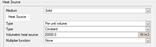
Double-click on Heat Source to open it in the detail
panel.
Change the Medium to Solid.
Click on the drop-down selector next to first Type option and select
Per unit volume.
This sets the type of heat source to volumetric heat
source.
Click on the drop-down selector next to the second Type option and select
Constant.
Set the Volumetric heat source value to 20000.0
W/m3
Figure 10.
Apply Volume Parameters
Volume groups are containers used for storing information about a volume region. This
information includes solution and meshing parameters applied to the volume and the
geometric regions that these settings are applied to.
When the geometry was imported into AcuConsole, all
volumes were placed into the "default" volume container.
In the next steps you will create volume groups for each volume in the model, assign
volumes to the respective volume groups, rename the default volume group container,
and set the materials and other properties for each volume group.
Expand the ModelData Tree item.
Create a new volume group for the solid inner cylinder.
Right-click on Volumes.
Click New.
Rename the new volume group to solid.
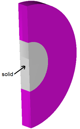
Add the solid component in the geometry to this group.
Right-click solid under Volumes in the Data Tree.
Click Add to.
Click the heating element portion of the geometry in the Visualization Area. Refer to the following figure to identify
the correct portion.
Figure 11.
Follow the instructions in the Add to dialog
if you need to manipulate the display to select the correct portion of
the geometry.
Click Done to add the selected volume to the
solid volume group.
Set up the solid volume element set.
The material model for this volume will be set to Stainless Steel, which is
the custom material model you created earlier in this tutorial, specifically for
this solid volume. Also the solid volume is to be set up as the heat
source
Expand the solid volume group in the tree.
Double-click Element Set to open the
Element Set detail panel.
Change the Medium to Solid.
Change the Material model to Stainless
Steel.
Change the Body force to Heat Source.
In the Data Tree, right-click on
default and rename it to
fluid.
Set up the Fluid volume element set.
Expand the fluid volume group in the tree.
Double click Element Set under fluid to open it
in the detail panel.
Ensure that the Medium for the volume is set to Fluid. If not, change
it to Fluid.
Change the Material model to Air.
Change the Body force to Gravity.
Create Surface Groups and Apply Surface Parameters
Surface groups are containers used for storing information
about a surface, including solution and meshing parameters, and the corresponding
surface in the geometry that the parameters will apply to.
In the next steps you will define surface groups,
assign the appropriate settings for the different characteristics of the problem,
and add surfaces to the group containers.
In the process of setting up a simulation, you need to move into different panels for
setting up the boundary conditions, mesh parameters, and so on, which can sometimes
be cumbersome, especially for models with too many surfaces. To make it easier, less
error prone, and to save time, two new dialogs are provided in AcuConsole. Use the Volume Manager and
Surface Manager to verify and provide the information for
all surface or volume entities at once. In this section some features of
Surface Manager are exploited.
Turn-off display for Volumes by right-clicking on
Volumes and selecting Display off
.
Right-click on Surfaces in the Data Tree and select Surface
Manager.
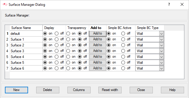
In the Surface Manager dialog, click New
six times to create six new surface groups.
Figure 12.
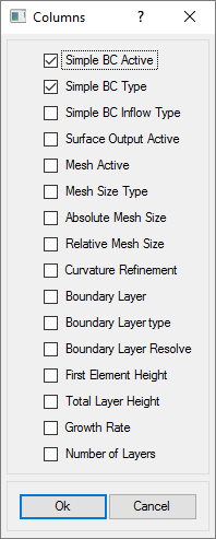
If you cannot see the Simple BC Active and Simple BC Type columns, click on
Columns , select these two columns from the list
and click Ok.
Figure 13.
Turn off the display for all surfaces except for the default surface.
Rename the default surface to inner_wall.
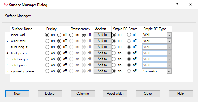
Rename Surface 1 through Surface 6 according to the image below.
Set the Simple BC Active and Simple BC Type columns as per Figure 14.
Figure 14.
Assign the periodic surfaces to the respective surface groups.
As mentioned earlier, the cylinders are assumed to be infinitely extended in
z-direction. Hence periodicity will be applied in this direction.
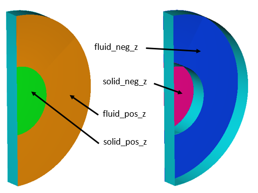
In the solid_pos_z row in the Surface Manager,
click Add to .
Select the planar symmetry surfaces as shown in Figure 15 and click Done.
Follow the procedure to assign all the surfaces that will extend in the
z-direction to respective surface collectors.
Figure 15.
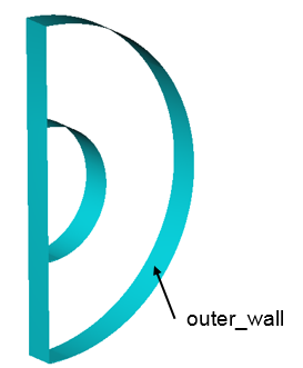
Assign the outer wall of the geometry to the outer_wall surface group. Use
Figure 16 as
the reference for selecting the required surfaces.
Figure 16.
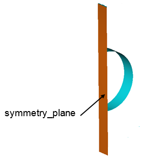
Assign the surface for symmetry_plane.
Figure 17.
When the geometry was loaded into AcuConsole,
all geometry surfaces were placed in the default surface group container. This
default surface group was renamed to inner_walls. In the previous steps, you
assigned some surfaces to various other surface groups that you created. At this
point, all that is left in the inner_walls surface group are the surfaces which make
up the contact boundary between the inner cylinder and the fluid
volume.
Close the Surface Manager.
Assign Surface Parameters
The modeling for this simulation was done using half symmetry. The model is only a
partial representation of the system, the complete geometry of which is a cylinder.
Hence it is appropriate to set the surface that you chose as symmetry_plane with a
symmetry boundary condition to simulate that effect.
This change was completed using the Surface Manager in the last
section. The following steps are thus optional.
Update symmetry_plane.
Expand the symmetry_plane surface in the tree.
Double-click Simple Boundary Condition under
symmetry_plane to open the Simple Boundary
Condition detail panel.
Ensure that the Type is set to Symmetry.
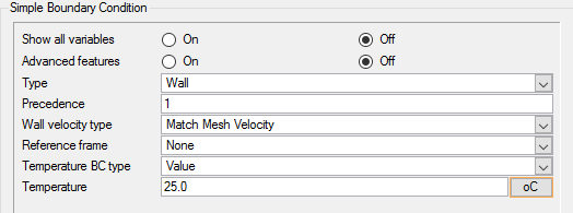
Update outer_wall.
Expand the outer_wall surface group in the tree.
Double click Simple Boundary Condition under
outer_wall to open the Simple Boundary Condition
detail panel.
Ensure that the Type is set to Wall.
Verify that the Wall velocity type is set to Match Mesh Velocity.
Change Temperature BC type from Flux to
Value.
Set the Temperature to 25° C.
The default unit for temperature input is K. You can change the unit
for temperature by clicking on the unit button at the right of the input
field, and selecting oC from the appearing menu. Figure 18.
Update inner_wall
The inner walls form the boundary surface of the inner cylinder volume, and
enclose the fluid volume on the inside. Since the inner cylinder is a solid
medium, this contact boundary will be a wall.
Expand the inner_wall surface group in the tree.
Double click Simple Boundary Condition under
inner_wall to open the Simple Boundary Condition
detail panel.
Ensure that the Type is set to Wall.
Verify Wall velocity type is set to Match Mesh Velocity.
Update the periodic surfaces solid_pos_z, solid_neg_z, fluid_pos_z, and
fluid_neg_z
Physically the simulation domain is assumed to extend infinitely in the
z-direction. However, only a small section of the cross section is being
modelled and the solution is assumed to be consistent along the z-direction.
Thus, these periodic surfaces are not physical boundaries but the solution on
these surfaces is constrained to be equal by periodicity. This is achieved via a
periodic boundary condition in AcuConsole, which
links the corresponding pairs of nodes on the two surfaces which are to be
constrained with a periodic boundary condition.
Periodicity can be defined
before proceeding with mesh generation. With this workflow, when the mesh is
generated, AcuMeshSim, which is the mesh
generation engine for AcuSolve, will read the
defined periodicity constraints and ensure a periodic mesh on the specified
surface pairs.
Expand the Model Data Tree item, and
right-click on Periodics.
Select New from the context menu to create a new
entity, Periodic 1.
Repeat the above step to create a second entity Periodic 2.
Rename the two new entities as periodicity_fluid
and periodicity_solid.
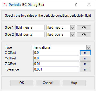
Right-click on periodicity_fluid and select
Define from the context menu.
In the Periodic BC dialog, make the following
settings.
Use the drop-down arrow to select the surfaces for Side 1 and
Side 2 as fluid_neg_z and
fluid_pos_z, respectively
Check that the Type is set to Translational.
Set X, Y and Z-offset as 0.0,
0.0, 0.01
respectively.
Use the following figure for reference for setting up the periodic
BC. Figure 19.
Click OK to close the dialog.
Using the same figure as reference, similarly define the periodic BC
for the entity periodicity_solid, with only the following changes:
Use the drop down arrows for Side 1 and Side 2 and select
solid_neg_z and
solid_pos_z, respectively.
Create Time History Output Points
Time History Output commands enables you to extract the nodal solution at any point
within the domain.
In the tree, double-click on Output, then right-click on
Time History Output, and select
New.
A new entry, Time History Output 1, will be created in the Data Tree under the Time History Output branch.
Right-click on Time History Output 1, select
Rename, and type in Monitor
points as the entity name.
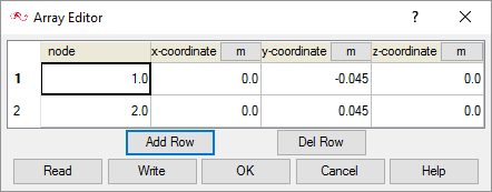
Double click Monitor points to open the detail panel. In
the detail panel,
Change the Type to Coordinates.
Click Open Array.
In the Array Editor, add a new row by clicking
Add Row.
Fill in the values as follows:
Figure 20.
Click OK.
Set Time step frequency to 1.
This will save the results for the defined time history points at every time
step.
Save the database.
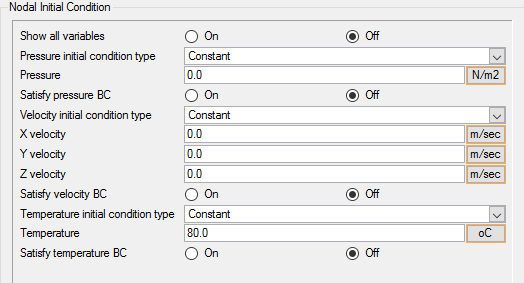
Set the Initial Conditions
Double-click on Nodal Initial Condition in the Data Tree to open the detail panel.
Set the Temperature to 80° C.
The default unit for temperature input is K. You can change the unit
for temperature by clicking on unit to the right
of the input field, and selecting oC from the
appearing menu.
Alternatively, enter 353.15 K in the temperature
field.
Figure 21.
Assign Mesh Controls
Set Global Mesh Parameters
Now that the flow characteristics have been set for the whole problem, a sufficiently
refined mesh has to be generated.
Global mesh attributes are the meshing parameters applied to the model as a whole
without reference to a specific geometric volume, surface, edge, or point. Local
mesh attributes are used to create mesh generation controls for specific geometry
components of the model.
In the next steps you will set the global mesh attributes.
Click MSH in the Data Tree Manager to filter the
settings in the Data Tree to show only the controls
related to meshing.
Double-click the GlobalData Tree item to expand it.
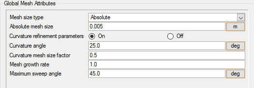
Double-click Global Mesh Attributes to open the
Global Mesh Attributes detail panel.
Change the Mesh size type to Absolute.
Enter 0.005 m for the Absolute mesh size.
Figure 22.
Set Surface Mesh Parameters
Surface mesh attributes are applied to a specific surface in the model. It is a
type of local meshing parameter used to create targeted mesh controls for one or
more specific surfaces.
Setting local mesh attributes, such as surface mesh attributes, is not mandatory.
When a local mesh attribute is not found for a component, the global attributes
are used as the mesh generation control for that component. If a local mesh
attribute is present, it will take precedence over the global setting.
In the next steps you will set the surface meshing attributes.
Go to the Solver Browser, expand 01.Global, then click
PROBLEM_DESCRIPTION.
Expand the ModelData Tree item.
Under the Model branch, expand the Surfaces. Under
Surfaces, expand the inner_wall surface group.
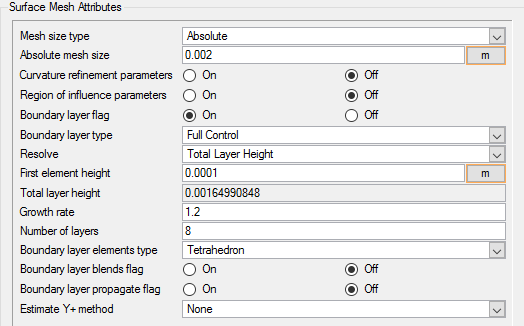
If necessary, check the box next to Surface Mesh
Attributes to activate it. Double-click it to open the
Surface Mesh Attributes detail panel.
The detail panel should now be populated with options related to the
local surface meshing controls.
Ensure that the Mesh size type is set to Absolute.
Enter 0.002 m for the Absolute mesh size.
Switch the Boundary layer flag to On.
Mesh controls related to boundary layer meshing become
visible.
Check the Boundary layer type is set to Full
Control.
Set Resolve to Total Layer Height.
This sets the total layer height based on the other settings you
provide.
Set the remaining settings as follows:
Option
Description
First element height
0.0001
Growth rate
1.2
Number of layers
8
Boundary layer elements type
Tetrahedron
Figure 23.
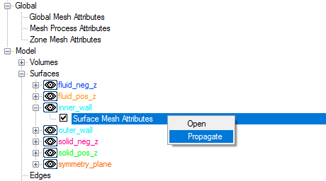
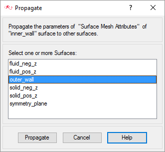
Instead of repeating the above steps for the outer_wall surface, you can
choose to propagate the mesh attribute settings for inner_wall surface group to
outer_wall surface group.
Under the inner_wall surface, right-click Surface Mesh
Attributes and select Propagate.
Figure 24.
In the Propagate dialog, select the surface
outer_wall and click
Propagate.
Figure 25.
Define Mesh Extrusion
The present simulation is equivalent to a 2D representation of the model, which
actually extends infinitely in both sides along the z-direction. In AcuSolve, 2D models are simulated by having just one element
across the faces of the cross section. Thus when these faces are set up with a
similar boundary condition, it coerces the corresponding nodes across the faces to
have same results. In this problem, these faces are the negative and positive
z-surfaces. This kind of mesh is achieved in AcuSolve
with mesh extrusion process. In the following steps, the process of extrusion of the
mesh between these surfaces is defined.
Expand the ModelData Tree item.
Right-click Mesh Extrusions and select
New from the context menu to create a new entity,
Mesh Extrusion 1.
Repeat the above step to create a second entity, Mesh Extrusion 2.
Rename the two entities as extrusion_fluid and
extrusion_solid.
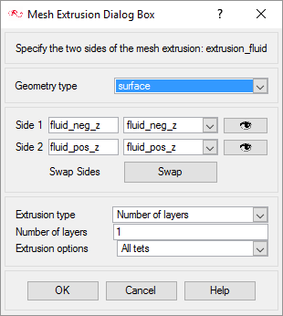
Right-click extrusion_fluid and select
Define from the context menu.
In the Mesh Extrusion dialog, make the following
settings.
Check that the Geometry type is set to surface.
Use the drop down arrows to select the surfaces for Side 1 and Side 2
as fluid_neg_z and
fluid_pos_z, respectively.
Check that the Extrusion type is set to Number of layers.
Set Number of layers equal to 1.
Set Extrusion options to All tets.
Use the following figure for reference for setting up the mesh extrusion for
extrusion_fluid. Figure 26.
Click OK to close the dialog.
Using the same figure as reference, similarly define the mesh extrusion for the
entity extrusion_solid, with only the following changes:
Use the drop down arrows to select the surfaces for Side 1 and Side 2
as solid_neg_z and
solid_pos_z, respectively
Generate the Mesh
In the next steps you will generate the mesh that will be used when computing a
solution for the problem.
Click on the toolbar to open the Launch
AcuMeshSim dialog.
For this case, the default settings will be used. Figure 27.
Click Ok to begin meshing.
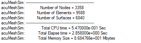
During meshing an AcuTail window opens. Meshing
progress is reported in this window. A summary of the meshing process indicates that the
mesh has been generated.
Figure 28.
Note: The actual number of nodes and elements, and memory usage may vary
slightly from machine to machine.
Visualize the mesh in the modeling window. Turn on
the display of surfaces and set the display type to solid and
wire.
Rotate and zoom in the model to analyze the various mesh regions.
Assign Reference Pressure
The present case does not have any inlet or outlet surfaces to define any boundary
condition that sets the pressure level inside the domain. To make the solution more
robust, you will set a pressure reference point using a nodal boundary condition.
The following steps will show how to setup the reference pressure inside the CFD
domain.
Click BAS in the Data Tree Manager to switch to basic view in the Data Tree.
Expand the ModelData Tree item.
Right-click on Nodes and select
New to create a new entity, Node 1.
Rename Node 1 to Fixed Pressure Node.
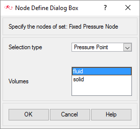
Right-click Fixed Pressure Node and select
Define.
In the Node Define Dialog Box, set Selection Type to
Pressure Point and Volumes to
fluid.
Figure 29.
Click OK.
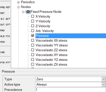
Expand Fixed Pressure Node and enable
Pressure.
The single node will now act as the pressure reference point for the
simulation. The default Type of Zero sets the nodes in this set to pressure =
0.0. Figure 30.
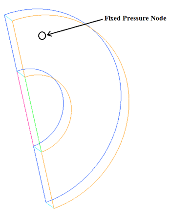
Examine the location of the reference pressure node and check that it is inside
the domain.
Right-click on Fixed Pressure Node and select
Display on.
Right-click on Surfaces and set Display type to
outline.
Right-click Periodics and select
Display off.
You should be able to see the fixed pressure node as a point, as shown
in the figure below. Figure 31.
Compute the Solution and Review the Results
Run AcuSolve
In the next steps you will launch AcuSolve to compute the solution for this case.
Click on the toolbar to open the
Launch AcuSolve dialog.
Click Ok to start the
solution process.
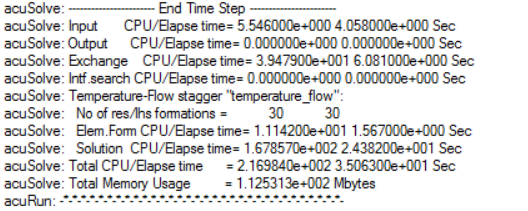
While computing the solution, an
AcuTail window opens. Solution progress is
reported in this window. A summary of the solution process indicates
that the run has been completed.
The information provided in the summary is based on
the number of processors used by AcuSolve.
If you use a different number of processors than indicated in this
tutorial, the summary for your run may be slightly different than the
summary shown.
Figure 32.
Close the AcuTail window and save the database to create a
backup of your settings.
Post-Process with AcuProbe
AcuProbe can be used to monitor various variables
over solution time.
Note: This solution was obtained by running AcuSolve
with four processors.
Open AcuProbe by clicking on the toolbar.
In the Data Tree on the left, expand
Residual Ratio. Right-click on Final
and select Plot All.
This will plot the residuals for the three variables, pressure,
temperature and velocity, in the plot area.
Note: You might need to click on the toolbar in order to
properly display the plot.
Figure 33.
Right-click on Final under Residual Ratio and select
Plot None.
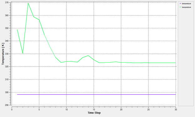
Expand Time History > Monitor Points.
Expand node 1 and node 2.
One node at a time, right-click on temperature and
select Plot.
Note: You might need to click on the toolbar in order to
properly display the plot.
Figure 34.
The node 1 lies in the bottom half of the model and the node 2 in the upper
half. The temperature distribution in the above plot shows that in steady
state upper half of the cylinder annulus is occupied by the hotter air and
lower half has the colder air.
In the menu area, click the
surfs collector and select
all.
The time series data of the variables can also be exported as a text file
for further post-processing.
Right-click on the variable that you want to export and click
Export.
Enter a File name and choose .txt for
the Save as type.
Click Save.
View Results with AcuFieldView
The tutorial has been written with the assumption that you have become familiar with the
AcuFieldView interface and basic operations. In general, it will
be helpful to understand the following basics:
How to find the data readers in the File menu and open up the desired reader panel for
data input.
How to find the visualization panels either from the toolbar or the Visualization panels
from the main menu to create and modify surfaces in AcuFieldView.
How to move the data around the modeling window using mouse
actions to translate, rotate and zoom in to the data.
This tutorial shows you how to work with steady state analysis data.
Start AcuFieldView
Click on the
AcuConsole toolbar to open the
Launch AcuFieldView dialog.
Click Ok to start
AcuFieldView.
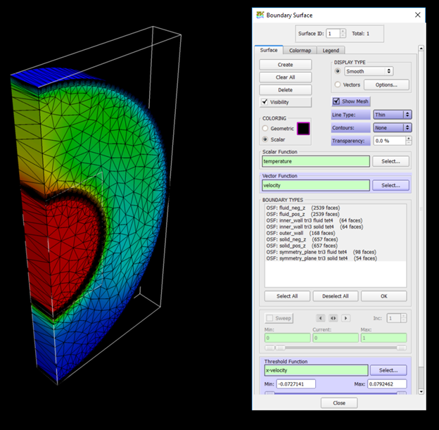
You will see that the temperature contours have already been displayed
on all the boundary surfaces with mesh. Figure 35.
Manipulate the Model View in AcuFieldView
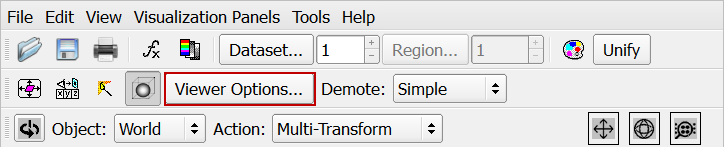
Close the Boundary Surface dialog.
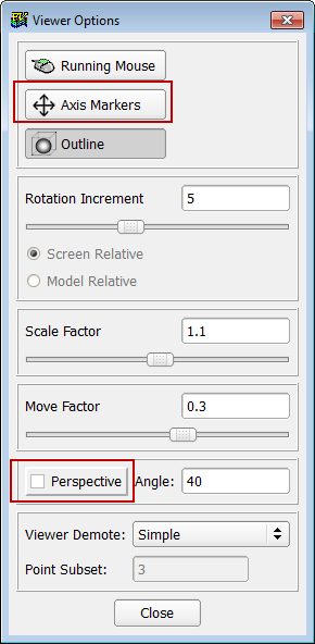
Click Viewer Options.
Figure 36.
Turn off perspective view by deselecting the Perspective
check box.
Disable axis markers by clicking on the Axis Markers
button.
Figure 37.
Close the Viewer Options dialog.
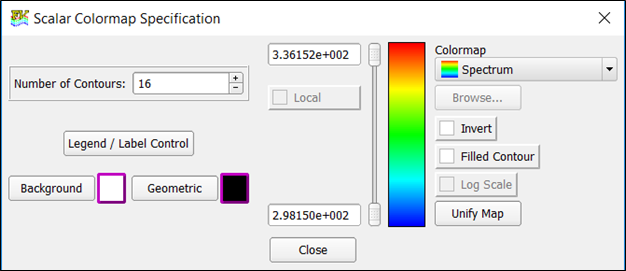
Click on the Colormap Specification icon on the toolbar.
Click on Background in the Scalar Colormap
Specification dialog and select white from the color palette that
opens.
Figure 38.
Close both dialogs.
Click on the Toggle Outline icon on the toolbar to turn off the
outline display.
Your AcuFieldView display should now look
like this. Figure 39.
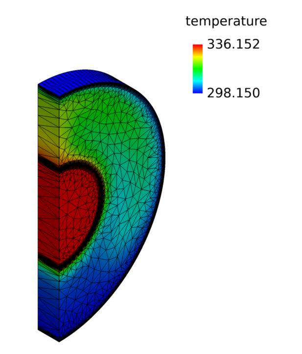
Create the Boundary Surface Showing Temperature for the Outer Surfaces with Mesh
Orient the geometry as shown in the figure below, so that the symmetry plane
and periodic surfaces are visible.
Click to open the Boundary
Surface dialog.
Click the Legend tab and check the Show
Legend check box.
Change the color of labels to black from the color palette.
If desired, change the number of labels to show more labels.
Change the Annotation title color to black.
Note: You can move the legend using Shift + left click,
and resize it using Shift + right click. Figure 40.
Coordinate the Surface Showing Temperature on the Mid-Coordinate Surface
In the Surface tab in the Boundary Surface dialog box,
click Visibility to turn it off.
Click Create to create a new Boundary Surface set.
Check Visibility to turn it on.
Set the Display Type to Outlines.
Under Boundary Types, click Select All, and click
Ok.
Click to open
the Coordinate Surface dialog.
Click Create to create a new Coordinate Surface.
Set the Coord Plane to Z.
The coordinate surface created is the mid plane between the two periodic
surfaces in the model.
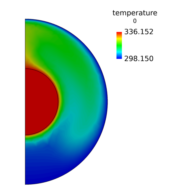
Change the Coloring to Scalar.
Set the Display Type to Smooth.
In the Scalar Function list, select Temperature as the
scalar function to be displayed.
In the Colormap tab, change Scalar Coloring to Local.
In the Legend tab, check the Show Legend check box to
display the temperature values on the coordinate plane.
From the Defined Views, select viewing direction as
+Z.
Figure 41.
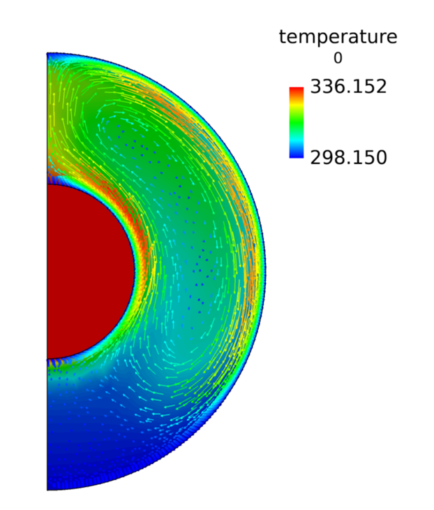
Coordinate the Surface Showing Vectors of Velocity on the Mid-Coordinate Surface
In the Surface tab in the Coordinate Surface dialog box,
click Create to create a new Coordinate Surface set.
Set the Display Type to Vectors.
Change the Coloring to Scalar.
In the Scalar Function list, select Velocity Magnitude
as the scalar function to be displayed.
Next to Vectors, click Options.
Activate Head Scaling and set it at
1.
Set the Length Scale to 4.
Activate the Skip option, and set the value to
50%.
Figure 42.
Summary
In this AcuSolve tutorial, you successfully set up and solved a
natural convection problem. The problem simulated a hot cylinder placed in the center of another
air-filled cylindrical volume. Air was modeled using a Boussinesq density approximation model,
which is used for buoyancy driven flows, such as those involving natural convection. As the film
of air in vicinity of the surface of the hot inner cylinder heated up, it generated convection
currents within the annular volume.
You started the tutorial by creating a database in AcuConsole,
importing and meshing the geometry and setting up the basic simulation parameters. The hot inner
cylinder was represented by a solid volume also acting as a heat source. Once the case was setup,
the solution was generated with AcuSolve.
Results were post-processed in AcuFieldView where you generated a
temperature profile, and a velocity vector profile, on a cross-section of the model.
New features that were introduced in this tutorial include creating and specifying a new custom
material in AcuConsole, specifying a volume group as a heat source
using the Boussinesq density model and setting up periodic boundary conditions.

 on the toolbar.
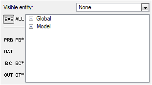
 next to the item name.
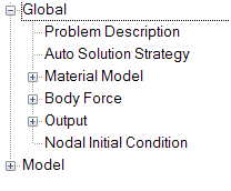
 on
the toolbar.
on
the toolbar.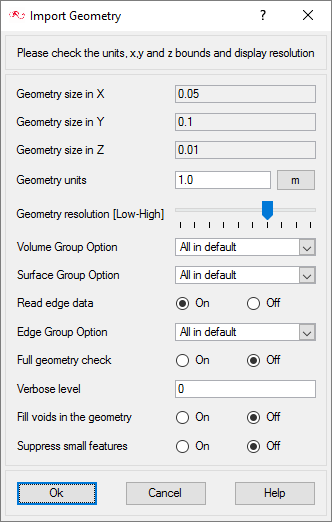

 on the toolbar to open the Launch
AcuMeshSim dialog.
For this case, the default settings will be used.
on the toolbar to open the Launch
AcuMeshSim dialog.
For this case, the default settings will be used.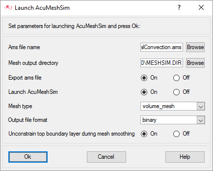
 on the toolbar to open the
Launch AcuSolve dialog.
on the toolbar to open the
Launch AcuSolve dialog.
 on the toolbar.
 on the toolbar in order to
properly display the plot.
on the toolbar in order to
properly display the plot.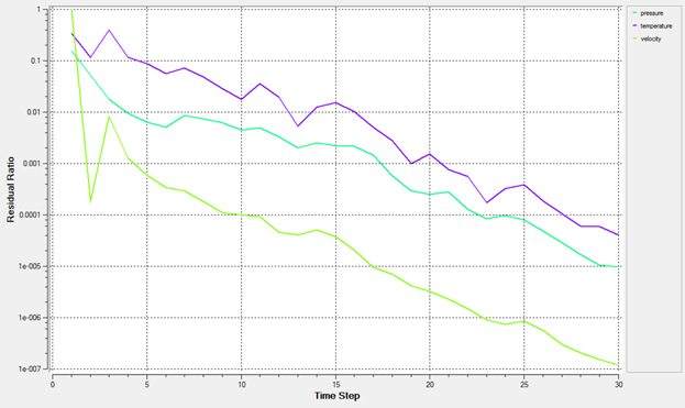
 on the
AcuConsole toolbar to open the
Launch AcuFieldView dialog.
on the
AcuConsole toolbar to open the
Launch AcuFieldView dialog.
 on the toolbar.
 on the toolbar to turn off the
outline display.
Your AcuFieldView display should now look like this.
on the toolbar to turn off the
outline display.
Your AcuFieldView display should now look like this.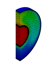
 to open the Boundary
Surface dialog.
to open the Boundary
Surface dialog.
 to open
the Coordinate Surface dialog.
to open
the Coordinate Surface dialog.