ACU-T: 2000 Turbulent Flow in a Mixing Elbow
Prerequisites
Prior to starting this tutorial, you should have already run through the introductory HyperWorks tutorial, ACU-T: 1000 HyperWorks UI Introduction. To run this simulation, you will need access to a licensed version of HyperMesh and AcuSolve.
Prior to running through this tutorial, copy HyperMesh_tutorial_inputs.zip from <Altair_installation_directory>\hwcfdsolvers\acusolve\win64\model_files\tutorials\AcuSolve to a local directory. Extract ACU-T2000_MixingElbow.hm from HyperMesh_tutorial_inputs.zip.
Since the HyperMesh database (.hm file) contains meshed geometry, this tutorial does not include steps related to geometry import and mesh generation.
Problem Description
The problem to be addressed in this tutorial is shown schematically in Figure 1. This is a typical industrial example for mixing in a pipe by injecting high-velocity fluid from a small inlet into relatively low-velocity fluid in the main pipe. It consists of a 90° mixing elbow with water entering through two inlets with different velocities. The geometry is symmetric about the XY midplane of the pipe, as shown in the figure

Figure 1. Schematic of Mixing Elbow
Open the HyperMesh Model Database
-
Click the Open Model icon
 located on the standard toolbar.
The Open Model dialog opens.
located on the standard toolbar.
The Open Model dialog opens.
Set the General Simulation Parameters
-
In the Entity Editor, set the Turbulence Model to
Spalart Allmaras.
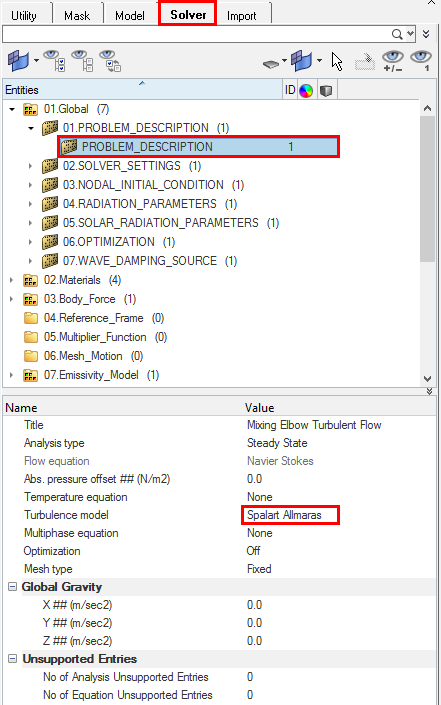
Figure 2.
Set Up Boundary Conditions
-
Click Large_Inlet. In the Entity Editor,
- Change the Type to INFLOW.
- Set the Inflow type to Average velocity.
- Set the Average velocity to 0.4 m/s.
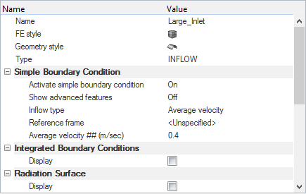
Figure 3. -
Click Outlet. In the Entity Editor, change the Type to OUTFLOW.
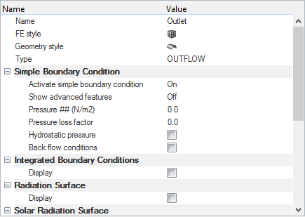
Figure 4. -
Click Symmetry. In the Entity Editor, change the Type to
SYMMETRY.
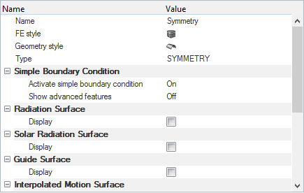
Figure 5. -
Click Wall. In the Entity Editor, verify that the Type is set to WALL.
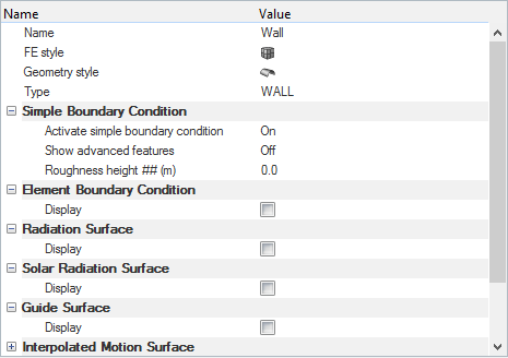
Figure 6. -
Click Fluid. In the Entity Editor,
- Change the Type to FLUID.
- Select Water_HM as the Material.
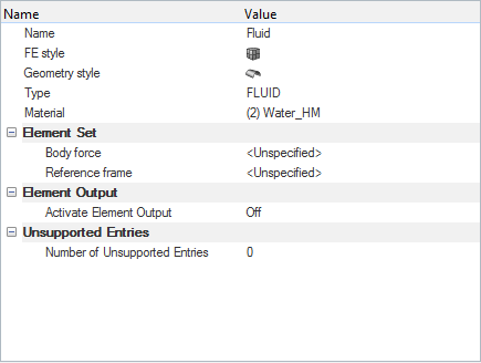
Figure 7.
Compute the Solution
In this step, you will launch AcuSolve directly from HyperMesh and compute the solution.
Run AcuSolve
-
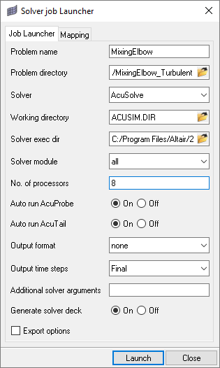
Click
 on the ACU toolbar.
The Solver job Launcher dialog opens.
on the ACU toolbar.
The Solver job Launcher dialog opens. -
Leave the remaining options as
default and click Launch to start the solution
process.
Post-Process the Results with HyperView
Open HyperView and Load the Model and Results
-
In the Load model and results panel, click
 next
to Load model.
next
to Load model.
Create Contour Plots of Pressure and Velocity
-
Click the Isolate Shown icon
 then click the Symmetry
component to turn off the display of all components in the graphics window
except the Symmetry component.
then click the Symmetry
component to turn off the display of all components in the graphics window
except the Symmetry component.
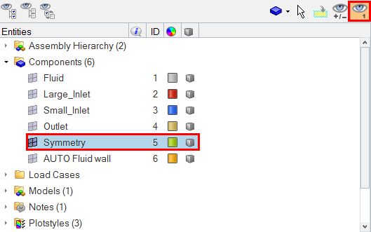
Figure 8. -
Orient the display to the xy-plane by clicking
 on the Standard Views toolbar.
-
Click
 on the Results toolbar to open the Contour panel.
-
In the panel area, under the Display tab, turn off
the Discrete color option.
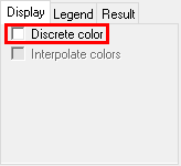
Figure 9. -
Click the Legend tab then
click Edit Legend. In the dialog, change the Numeric
format to Fixed then click
OK.
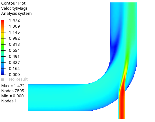
Figure 10. -
Change the result type to Pressure(s) then click
Apply to view the pressure contour on the symmetry
plane.
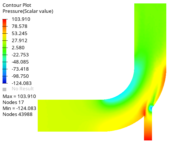
Figure 11.
Summary
In this tutorial, you worked through a basic workflow to set up a CFD model, carry out a CFD simulation, and post-process the results using HyperWorks products, namely AcuSolve, HyperMesh, and HyperView. You started by importing the model in HyperMesh. Then, you defined the simulation parameters and launched AcuSolve directly from within HyperMesh. Upon completion of the solution by AcuSolve, you used HyperView to post-process the results and create contour plots.