AcuPlotData
Plotting utility for basic two-dimensional plot creation from an ascii text data file.
Syntax
acuPlotData [options]
Type
AcuSolve Post-Processing Program
Description
AcuPlotData is a post-processing utility that uses generic ascii text data files as input to generate two-dimensional visualizations based on the functionality available in the Python library, Matplotlib. AcuPlotData is provided to AcuSolve users for the purpose of generating high-quality visualizations of AcuSolve outputs leveraging automated input and image processing. You are required to provide an ascii text file defined with the files attribute. Further control of the image development process is achieved using the input commands that are able to customize the visualization for user specific requirements.
In the following, the full name of each option is followed by its abbreviated name and its type. For a general description of option specifications, see Command Line Options and Configuration Files. See below for more individual option details:
- help or h (boolean)
- If set, the program prints a usage message and exits. The usage message includes all available options, their current values, and the place where each option is set.
- problem or pb (string)
- The name of the problem is specified via this option. This name is used to generate input file names and extracted surface file names.
- files (string)
- Comma-separated list to specify the files used to generate plots from. Defines the files that will be plotted, one or more files are required at input. The files attribute should reference file names that each contain rows of data with format, row index, x, y, z (using any delimiter). Quantities are not restricted to any specific number of columns or data type (real and integer are accepted).
- x_column or x_col (int)
- Specifies the x_column (abscissa axis) of the data file to be plotted as the independent variable. Accepts a single column for all y_columns provided by you.
- y_columns or y_cols (string)
- Comma-separated list to specify the y-column places to be plotted. Each integer in the list specifies the y_column (ordinate axis) of the data file to be plotted as the dependent variable(s). Accepts one or more columns separated by commas for all y_columns provided by you.
- x_scale_factor or x_scale (real)
- Specifies the x-scale factor to apply to plotted data. Multiplies the x_column data by x_scale_factor.
- y_scale_factors or y_scale (str)
- Comma-separated list to specify the y-scale factor(s) to apply to plotted data. Multiplies the y_columns data by y_scale_factor once separated from the list. Only provide a single value when one value for y_columns is given.
- offset (real)
- Specifies the percentage of initial data points to skip when plotting the data file.
- fft (boolean)
- If this option is set to True, time dependent data will be transformed using a Fast-Fourier transformation. If using, the first column in the data file must be time, as this is used to compute the time-step size and subsequent quantities in relation to the FFT.
- stats (boolean)
- If this option is set to True, basic statistical quantities will be computed from the user provided y_colunms fields. The application will compute the maximum, minimum, mean, and root-mean-square (rms) of data.
- type or plot_type (enumerated)
- Specifies the format of the vertical and horizontal axes. When plot_type=standard, each axis is plotted with a linear range of points. semilogx, semilogy and loglog will specify that the horizontal, vertical or both axes are plotted using a logarithmic distribution of the data, respectively.
- x_axis_range or x_range (string)
- Comma-separated string to specify the minimum and maximum range of the horizontal axis. When not issued, the plot will automatically select the minimum and maximum viewable region. You can also input “tight” to automatically select the viewable range, with tighter overlap on both sides of the plot.
- y_axis_range or y_range (string)
- Comma-separated string to specify the minimum and maximum range of the vertical axis. When not issued, the plot will automatically select the minimum and maximum viewable region. You can also input “tight” to automatically select the viewable range, with tighter overlap on both sides of the plot.
- x_axis_invert or x_invert (boolean)
- If this option is set to True, the horizontal (x) axis will be inverted.
- y_axis_invert or y_invert (boolean)
- If this option is set to True, the vertical (y) axis will be inverted.
- x_tick_range or x_ticks (string)
- Comma-separated string to specify the ticks on the horizontal axis. Provided as x-minimum, x-maximum, increment (no spaces). When not issued, the plot will automatically select the horizontal tick locations.
- y_tick_range or y_ticks (string)
- Comma-separated string to specify the ticks on the vertical axis. Provided as y-minimum, y-maximum, increment (no spaces). When not issued, the plot will automatically select the vertical tick locations.
- marker_size or ms (string)
- Comma-separated string to specify the size of each of the markers in points provided by the y_columns attribute.
- marker_edge_width or mew (real)
- Specifies the edge width size of each of the markers provided by the y_columns attribute.
- marker_face_color or mfc (string)
- Comma-separated string to specify the color of each marker face provided by the y_columns attribute. Set to w for non-filled markers.
- marker_edge_color or mec (string)
- Comma-separated string to specify the color of each marker edge provided by the y_columns attribute. Set to w for no marker edge.
- draw_legend or dl (boolean)
- If this option is set to True, a legend representing each of the data columns provided by the y_columns attribute will be added to the plot.
- legend or leg (string)
- Comma-separated string to specify legend contents, with each entry added as a separate line in the legend.
- legend_size or leg_size (int)
- Font size for legend text.
- legend_location or leg_loc (enumerated)
- Specifies the location of the legend if draw_legend=true. The following options for the location are available; best, center, lower_left, center_right, upper_left, center_left, upper_right, lower_right, upper_center, lower_center.
- line_format or lfmt (string)
- Comma-separated string to specify the line formats assigned to the data provided by the y_columns attribute. The following options for the format of the line are available; _auto, (markers=- -- + o . , s v x < >, colors = b g r c m y k w 0.75. Markers may be combined with other markers and colors to define the line/marker configuration (--o for dashed dotted line).
- line_width or lw (string)
- Comma-separated string to specify the line and point width(s) assigned to the data provided by the y_columns attribute.
- title_string or title (string)
- Specifies the name of the title on the plot.
- title_size or tsize (integer)
- Specifies the size of the title on the plot.
- x_label (string)
- Specifies the label for the horizontal axis of the plot.
- y_label (string)
- Specifies the label for the vertical axis of the plot.
- label_size or lsize (integer)
- Specifies the size of the labels on the plot.
- tick_label_size or tlsize (integer)
- Specifies the size of the tick labels on the plot.
- axis_line_width or alw (integer)
- Specifies the size of the axis width on the plot.
- draw_grid or grid (boolean)
- If this option is set to True, a vertical and horizontal background grid will be drawn at the tick locations assigned in x_tick_range and y_tick_range.
- font (enumerated)
- Specifies the type of font used for the plot text. Available fonts are serif, sans-serif, cursive, fantasy and monospace.
- tex or latex_flag (boolean)
- If this option is set to True, the application will attempt to use LaTex to render strings.
- note_string or note (string)
- If this option is specified, the application will write the user requested note_string on the plot.
- note_size or nsize (integer)
- Specifies the size of the text written when note_string=”string”.
- note_loc or nloc (string)
- Specifies the location where the user requested note_string will be written on the plot. The location is specified in screen coordinates.
- plot_to_file or ptf (boolean)
- If this option is set to True, the plot will be saved to a file. The file name will be created dynamically based on the problem_name and output_format attributes.
- output_format or ofmt (string)
- Specifies the image file type extension when plot_to_file=true. The default is pdf.
- plot_to_screen or pts (boolean)
- If this option is set to True, the plot will be displayed during the application execution.
- num_time_steps or steps (integer)
- Specifies the number of timesteps when making time-dependent plots for animations.
- ignore_missing_files or imf (boolean)
- If this option is set to True, the application will ignore any missing files that are provided by the files attribute.
- verbose or v (integer)
- Set the verbose level for printing information to the screen. Each higher verbose level prints more information. If verbose is set to 0 (or less), only warning and error messages are printed. If verbose is set to 1, basic processing information is printed in addition to warning and error messages. This level is recommended. verbose levels greater than 1 provide information useful only for debugging.
Examples
acuPlotData -files diffuser.interp.dat,pb-c4.dat,pbot-exp.dat -y_cols 4 -x_scale
22.7272 -y_label "p/p_stag" -x_label x/H -title "Diffuser - Lower Surface Pressure"
-legend "AcuSolve,NASA Reference,Experiment" -pb diffuser_lower_pressure -lfmt
or,ob,ow -ms 1,5,5 -mec r,b,k -lw 2,2,2acuPlotData.pb=diffuser_lower_pressure
acuPlotData.files=diffuser.interp.dat,pb-c4.dat,pbot-exp.dat
acuPlotData.y_cols=4
acuPlotData.ptf=on
acuPlotData.x_scale=22.7272
acuPlotData.y_label="p/p_stag"
acuPlotData.x_label=x/H
acuPlotData.title="Diffuser - Lower Surface Pressure"
acuPlotData.legend="AcuSolve,NASA Reference,Experiment"
acuPlotData.lfmt=or,ob,ow
acuPlotData.ms=1,5,5
acuPlotData.mec=r,b,k
acuPlotData.lw=2,2,2acuPlotData: Plotting frame <1>
acuPlotData: Evaluating argument <diffuser.interp.dat>
acuPlotData: Found <1> files
acuPlotData: Processing file <diffuser.interp.dat>
acuPlotData: Plotting <500> points
acuPlotData: Evaluating argument <pb-c4.dat>
acuPlotData: Found <1> files
acuPlotData: Processing file <pb-c4.dat>
acuPlotData: Plotting <26> points
acuPlotData: Evaluating argument <pbot-exp.dat>
acuPlotData: Found <1> files
acuPlotData: Processing file <pbot-exp.dat>
acuPlotData: Plotting <36> points
acuPlotData: Printing plot to file <diffuser_lower_pressure.png>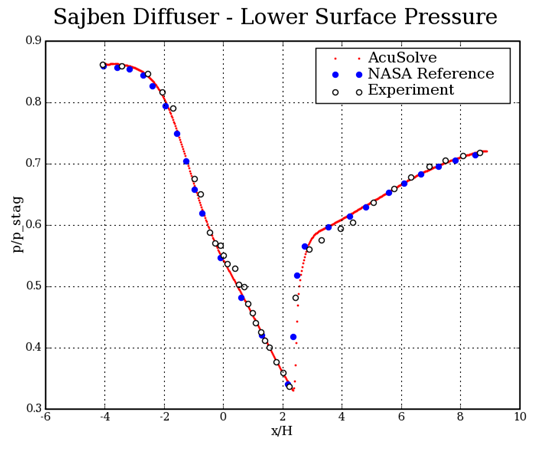
Figure 1.
acuPlotData -files exp.dat,sa.dat,sst.dat,ko.dat,rke.dat -y_cols 4 -y_label "Cf" -
x_label “Horizontal Location (m)” -title "Skin Friction Coefficient in an
Axisymmetric Diffuser" -legend "Experimental,AcuSolve-SA,AcuSolve-SST,AcuSolve-K-
Omega,AcuSolve-RKE" -lfmt ok,-r,-b,-g,-c -ms 2,1,1,1,1 -lw 2,2,2,2,2acuPlotData.pb=dr
acuPlotData.files= exp.dat,sa.dat,sst.dat,ko.dat,rke.dat
acuPlotData.y_cols=4
acuPlotData.ptf=on
acuPlotData.y_label="Cf"
acuPlotData.x_label=”Horizontal Location (m)”
acuPlotData.title="Skin Friction Coefficient in an Axisymmetric Diffuser"
acuPlotData.legend=Experimental,AcuSolve-SA,AcuSolve-SST,AcuSolve-K-Omega,AcuSolve-RKE
acuPlotData.lfmt= ok,-r,-b,-g,-c
acuPlotData.ms=2,1,1,1,1
acuPlotData.lw=2,2,2,2,2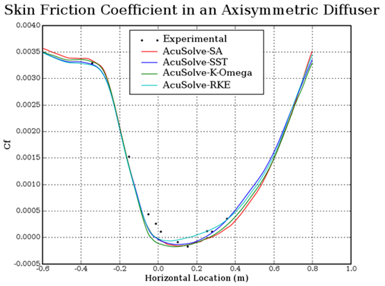
Figure 2.