ACU-T: 6104 AcuSolve - EDEM Bidirectional Coupling with Non-Spherical Particles
This tutorial introduces you to the workflow for setting up and running a basic bidirectional coupling (two-way) simulation with non-spherical particles using AcuSolve and EDEM. Prior to starting this tutorial, you should have already run through the introductory HyperWorks tutorial, ACU-T: 1000 Basic Flow Set Up, and have a basic understanding of HyperWorks CFD, AcuSolve, and EDEM. To run this simulation, you will need access to a licensed version of HyperWorks CFD, AcuSolve, and EDEM.
Prior to running through this tutorial, copy HyperWorksCFD_tutorial_inputs.zip from <Altair_installation_directory>\hwcfdsolvers\acusolve\win64\model_files\tutorials\AcuSolve to a local directory. Extract ACU-T6104_sieve.hm and sieve.dem from HyperWorksCFD_tutorial_inputs.zip.
Problem Description
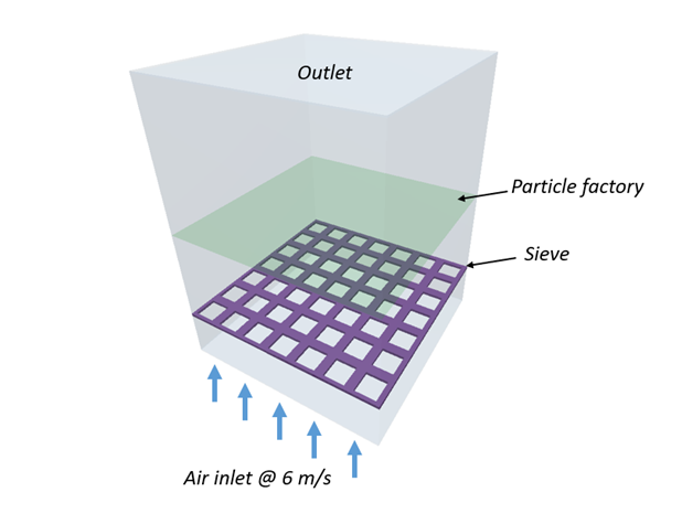
Figure 1.

Figure 2.
AcuSolve-EDEM bidirectional coupling is used to model the interaction between the fluid and particles. In this tutorial, non-spherical drag force models are used to accurately predict the drag forces on the particles by taking the shape of particles into consideration. The length scale used for factoring in the shape of the particles is the aspect ratio. Bar shaped particles with an aspect ratio of 2.75 and spherical particles with aspect ratio 1 are used for this simulation. The Rong drag model is used in conjunction with the Holzer-Sommerfeld non-spherical drag coefficient model.
The particle properties used for this simulation are listed in the table below:
| Particle Type | Density (kg/m3) | Size (m) | Number of particles |
|---|---|---|---|
| Bar | 200 | 0.022/0.008 (L/D) | 100 |
| Sphere | 1500 | 0.008 (D) | 200 |
Part 1 - EDEM Simulation
Start Altair EDEM from the Windows start menu by clicking .
Open the EDEM Input Deck
-
In the dialog, browse to your problem directory and open the
sieve.dem file.
The geometry is loaded.
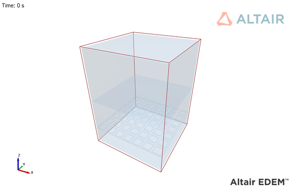
Figure 3.
Define the Bulk Materials and Equipment Material
In this step, you will define the material models for the bar and sphere-shaped particles.
-
Click
 below Interaction to define the
interaction properties for collisions among the bar shaped particles. In the
dialog, click OK.
below Interaction to define the
interaction properties for collisions among the bar shaped particles. In the
dialog, click OK.
-
Set the interaction coefficients as shown in the figure below.
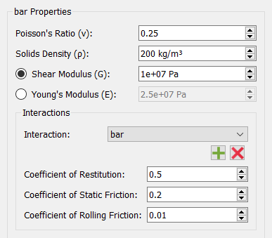
Figure 4. -
In the bar Spheres panel, set the Physical Radius and the XYZ positions as
shown in the figure below.
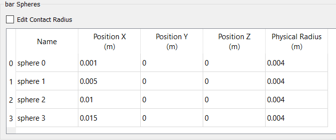
Figure 5. -
In the Creator Tree, click Calculate Properties.
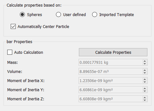
Figure 6.Note: Since the "Automatically Center Particle" option is active, EDEM will internally adjust the positions of the spheres in the particle. Although you might see minor changes in the location of the spheres, the overall dimensions of the particle stay the same. -
Click below Interaction to define the
interaction properties for collisions with sphere particles. In the dialog,
select sphere then click OK.
-
Set the interaction coefficients as shown in the figure below.
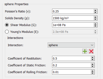
Figure 7. -
Click again to define the interaction
properties for collisions with bar particles. In the dialog, select
bar then click OK.
-
Set the interaction coefficients as shown in the figure below.
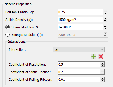
Figure 8. -
In the sphere Spheres panel, set the Physical Radius of the sphere to
0.004 m then press Enter.
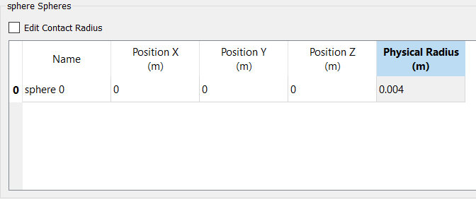
Figure 9. -
In the Creator Tree, click Calculate Properties.
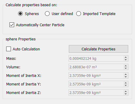
Figure 10. -
Click below Interaction to define the
interaction properties for collisions with bar particles. In the dialog, select
bar then click OK.
-
Set the interaction coefficients as shown in the figure below.
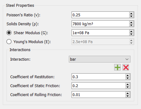
Figure 11. -
Click again to define the interaction
properties for collisions with sphere particles. In the dialog, select
sphere then click OK.
-
Set the interaction coefficients as shown in the figure below.
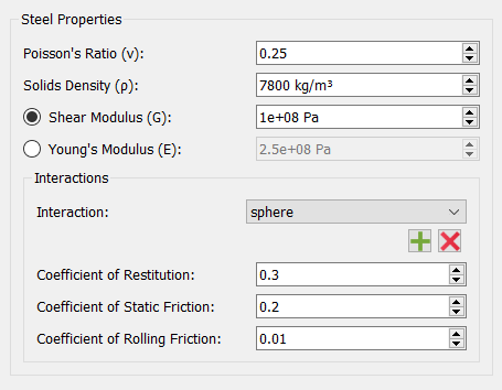
Figure 12.
Define Geometries and Factories
-
Name it oscillation and specify the parameters as shown
in the figure below.
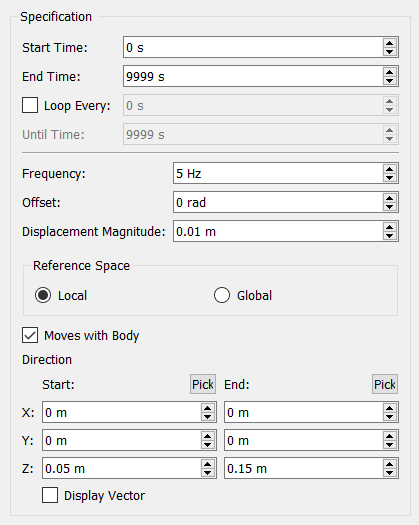
Figure 13. -
Set the particle generation parameters as shown in the figure below.
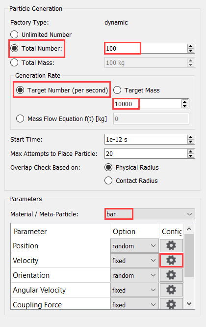
Figure 14. -
Click
 besides Velocity, set the
Z-velocity to -1 m/s, then click
OK.
besides Velocity, set the
Z-velocity to -1 m/s, then click
OK.
Define the Environment
In this step, you will define the extents of the domain for the EDEM simulation and the direction of gravitational acceleration.
Define the Simulation Settings
-
Click
 in the top-left corner to go to
the EDEM Simulator tab.
in the top-left corner to go to
the EDEM Simulator tab.
-
Set the Selected Engine to CPU Solver and set the Number
of CPU Cores based on availability.
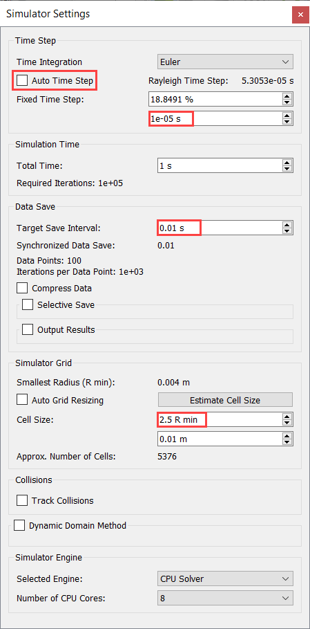
Figure 15.
Part 2 - AcuSolve Simulation
Start HyperWorks CFD and Open the HyperMesh Database
-
From the Home tools, Files tool group, click the Open Model tool.

Figure 16.The Open File dialog opens.
Validate the Geometry
The Validate tool scans through the entire model, performs checks on the surfaces and solids, and flags any defects in the geometry, such as free edges, closed shells, intersections, duplicates, and slivers.
Figure 17.
Set Up Flow
Set the General Simulation Parameters
-
From the Flow ribbon, click the Physics tool.

Figure 18.The Setup dialog opens. -
In the Material Library dialog, select EDEM 2 Way
Multiphase, switch to the My Material
tab, then click
 to add a new material model.
-
Set the Non spherical drag coefficient model to
Holzer-Sommerfeld.
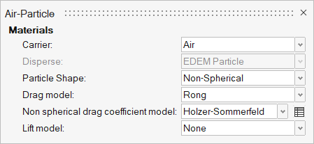
Figure 19. -
In the new dialog, click
 to add a new row, then enter the values for Aspect Ratio and Volume as shown in
the figure below.
to add a new row, then enter the values for Aspect Ratio and Volume as shown in
the figure below.
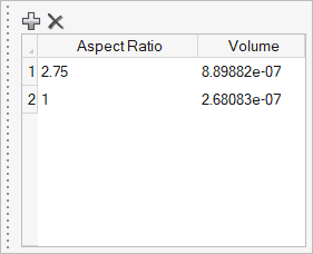
Figure 20.Note: The volumes entered here should be obtained from EDEM under particle properties. There might be slight variation in the volume values that you may see in your EDEM model but that is fine.Here the aspect ratios are calculated based on the ratio of the length to diameter of the particles. The AR of 2.75 and 1 are for bar and sphere-shaped particles respectively. The volume of the particles can be obtained from EDEM under the particle properties. If the simulation has particles of a single shape, then the volume field can be set to zero.
-
Set the Pressure scale to Absolute.
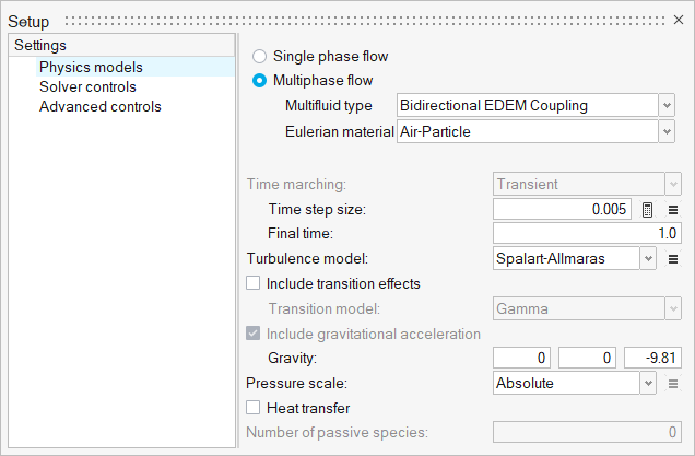
Figure 21. -
Click the Solver controls setting and set the Maximum
stagger iterations to 3.
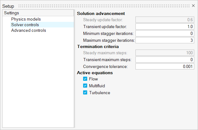
Figure 22.
Assign Material Properties
-
From the Flow ribbon, click the Material tool.

Figure 23. -
On the guide bar, click
 to exit
the tool.
to exit
the tool.
Define Flow Boundary Conditions
-
From the Flow ribbon, Profiled
tool group, click the Profiled Inlet tool.

Figure 24. -
Click on the inlet face highlighted in the figure below. In the microdialog, enter a value of 6 m/s
for the Average velocity and 1.0 for the Carrier fluid
volume fraction.
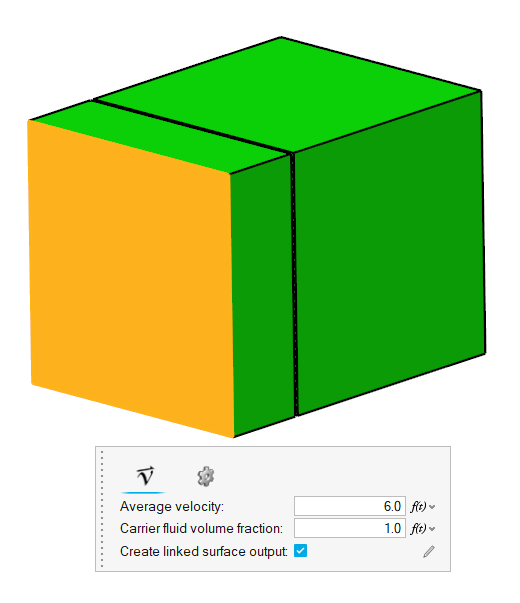
Figure 25. -
On the guide bar, click
 to execute
the command and exit the tool.
to execute
the command and exit the tool.
-
Click the Outlet tool.

Figure 26. -
Select the face highlighted in the figure below then click on the
guide bar.
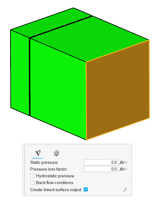
Figure 27.
Set Up Motion
Select the Motion Type
-
From the Motion ribbon, click the Settings tool.
Figure 28.
Define the Mesh Boundary Conditions
-
From the Motion ribbon, click the Planar Slip tool.

Figure 29. -
Select the two surfaces highlighted in the figure below.
The surfaces selected have the minimum y-coordinate.
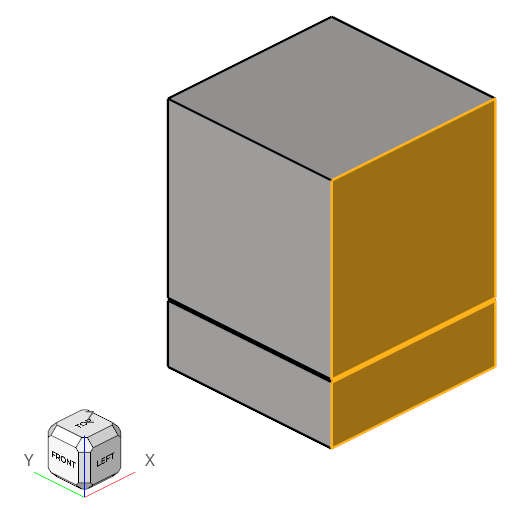
Figure 30. -
On the guide bar, click
 to execute the command and remain in the
tool.
to execute the command and remain in the
tool.
-
Repeat steps 2-4 to create three more planar slip boundary conditions for the
surfaces with the maximum y-coordiates, and the minimum and maximum
x-coordinates. Name these groups y_pos,
x_neg, and x_pos
respectively.
Once the four planar slip conditions are defined, the Mesh Motion legend should look like the one shown below.
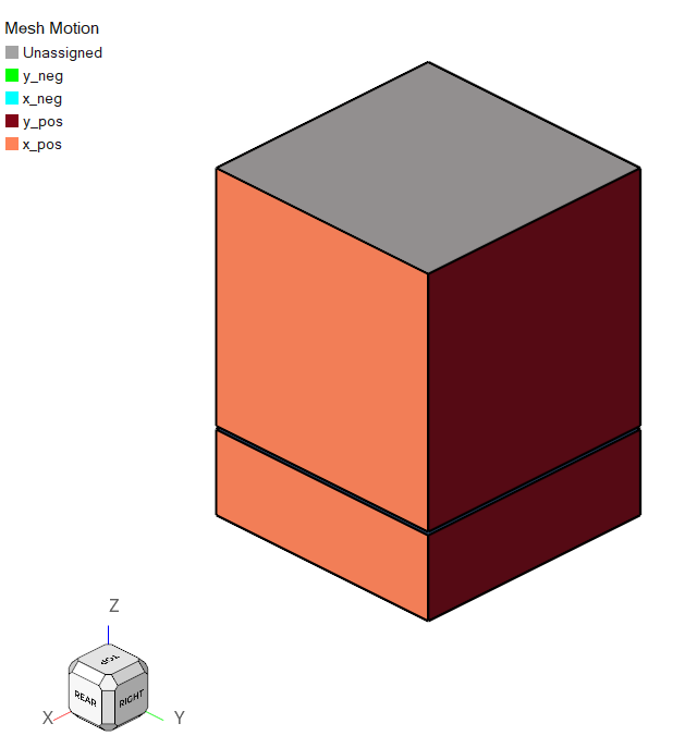
Figure 31.
Define Sinusoidal Translational Motion
-
From the Motion ribbon, click the Translation tool.

Figure 32. -
Using box selection, select all the sieve surfaces as shown in the figure
below.
Ensure that you are not selecting the inlet or outlet faces.
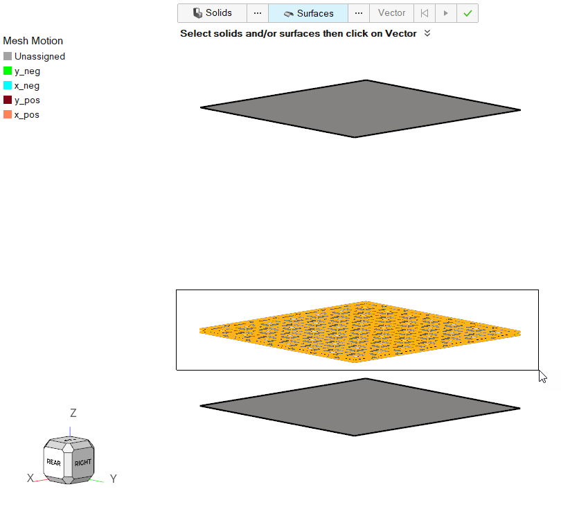
Figure 33. -
In the microdialog, click Z to
align the axis to the global z axis.
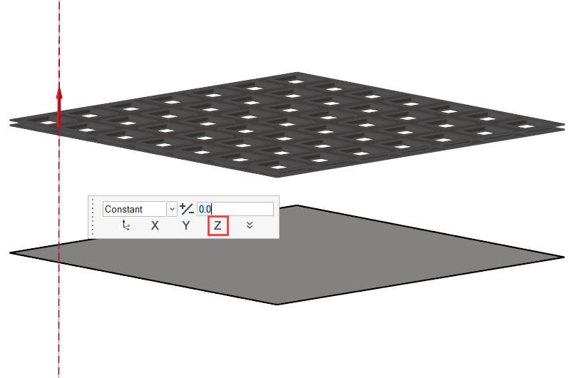
Figure 34. -
In the microdialog, change the type to
Time-varying and click the plot icon.
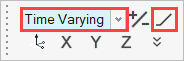
Figure 35. -
In the new plot dialog, click on the drop-down beside the table icon for
function specification and select the oscillating option.
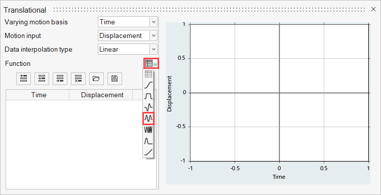
Figure 36. -
Enter the values for the sine function as shown in the figure below.
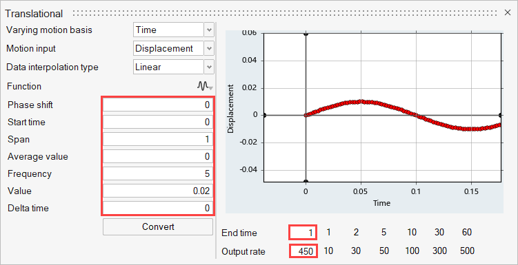
Figure 37. -
Click Convert to transform the sine function into an
array for the multiplier function.
The motion profile for the translation motion should look like the one shown below.
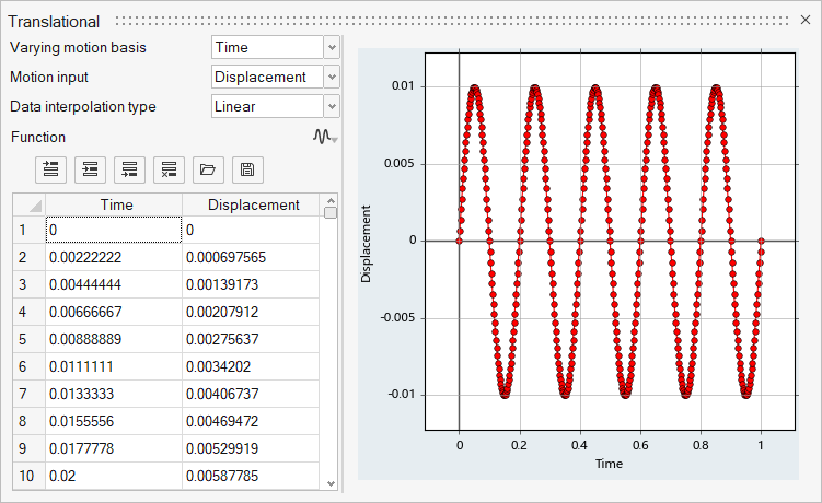
Figure 38. -
Click on the guide bar.
Generate the Mesh
-
From the Mesh ribbon, click the
Volume tool.

Figure 39.The Meshing Operations dialog opens. -
Set the Mesh size to Maximum size and change the Maximum
element size to 0.03.
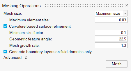
Figure 40.
Define Nodal Outputs
Once the meshing is complete, you are automatically taken to the Solution ribbon.
-
From the Solution ribbon, click the Field tool.

Figure 41.The Field Output dialog opens. -
Set the Time step interval to 0.05.
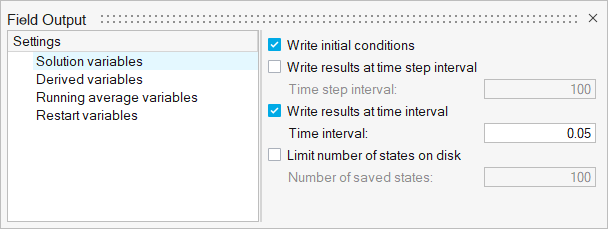
Figure 42.
Submit the Coupled Simulation
-
Start the coupling server by clicking Coupling Server in
EDEM.
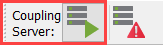
Figure 43.Once the Coupling server is activated, the icon changes.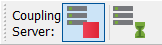
Figure 44. -
From the Solution ribbon, click the Run tool.

Figure 45.The Launch AcuSolve dialog opens. -
Click Run to launch AcuSolve.
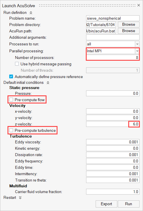
Figure 46.Once the AcuSolve run is launched, the Run Status dialog opens. -
In the dialog, right-click on the AcuSolve run and
select View log file.
If the coupling with EDEM is successful, that information is printed in the log file.
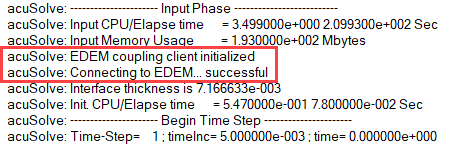
Figure 47.Once the simulation is complete, the summary of the run time is printed at the end of the log file.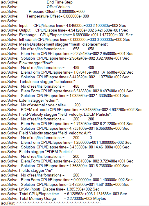
Figure 48.
Analyze the Results
AcuSolve Post-Processing
-
In HyperWorks CFD, right-click on the AcuSolve run in the Run Status
dialog and select Visualize results.
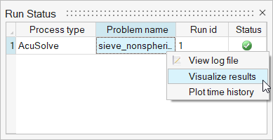
Figure 49.The results are loaded in the Post ribbon. -
Click the Slice Planes tool.

Figure 50. -
Select the x-z plane as highlighted in the figure below.
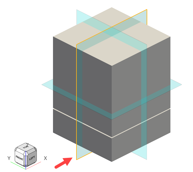
Figure 51. -
In the slice plane microdialog, click
 to
create the slice plane.
to
create the slice plane.
-
Click
 and set the Colormap name to Rainbow
Uniform.
and set the Colormap name to Rainbow
Uniform.
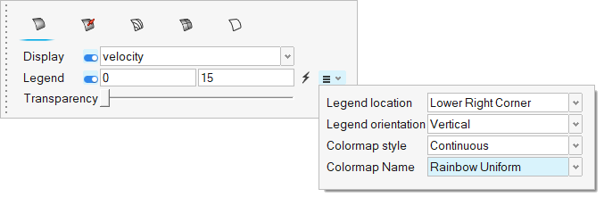
Figure 52. -
Click on the guide bar.
-
In the Post Browser, turn off the visibility of
Flow Boundaries by clicking on its icon.
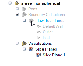
Figure 53. -
Select the Left face on the view cube to align the model
to the x-z plane.
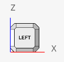
Figure 54. -
Click
 on the animation toolbar to view the animation of
the temperature contour.
on the animation toolbar to view the animation of
the temperature contour.
Figure 55. -
Click on the guide bar.
-
Click to start the animation.
Figure 56.
EDEM Post-Processing
-
Once the EDEM simulation is complete, click
 in the top-left corner to go to
the EDEM Analyst tab.
in the top-left corner to go to
the EDEM Analyst tab.
-
Verify that the Display Mode is set to Filled and set
the Opacity to 0.2.
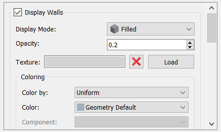
Figure 57. -
Click Apply All.
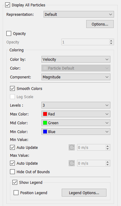
Figure 58. -
On the menu bar, set the time to
0 by clicking:

Figure 59. -
Set the View plane to + Y.
Figure 60. -
In the Viewer window, set the Playback Speed to 0.1x and
then click
 to play the particle flow animation.
Figure 61.Observe that the lighter bar shaped particles are blown away by the incoming fluid while the heavier particles fall through the sieve openings.
Summary
In this tutorial, you learned how to set up and run a basic AcuSolve-EDEM bidirectional (two-way) coupling problem with non-spherical particles. You learned how to create a non-spherical particle in EDEM and set up the AcuSolve model to consider the effect of the particle shape for the fluid-particle interaction forces. Once the simulation was complete, you learned how to post-process the AcuSolve results using HyperWorks CFD and the EDEM results.