ACU-T: 3300 Modeling of a Heat Exchanger Component
This tutorial provides instructions for modeling a heat exchanger component using HyperWorks CFD. Prior to starting this tutorial, you should have already run through the introductory tutorial, ACU-T: 1000 Basic Flow Set Up, and have a basic understanding of HyperWorks CFD and AcuSolve. To run this simulation, you will need access to a licensed version of HyperWorks CFD and AcuSolve.
Prior to running through this tutorial, copy HyperWorksCFD_tutorial_inputs.zip from <Altair_installation_directory>\hwcfdsolvers\acusolve\win64\model_files\tutorials\AcuSolve to a local directory. Extract ACU-T3300_HeatExchanger.hm from HyperWorksCFD_tutorial_inputs.zip.
Problem Description
Heat exchangers are devices used to facilitate heat exchange between two fluids that are at different temperatures. A typical heat exchanger device has two separate flows, the cross flow and tubular flow. Depending on the temperatures, heat can flow to or from one fluid to the other through the solids separating them. Since the heat exchanger geometry is quite complex with a large number of plates and pipes, it is not realistic to model the actual heat exchanger when performing system level simulations. In such scenarios, a simplified approach can be employed where only the effect of the heat exchanger on the cross flow is considered instead of modeling the actual heat exchanger. This is done using the heat exchanger component available in AcuSolve.
The heat exchanger component has two effects on the cross flow:
- Pressure drop which is calculated based on the friction parameters provided by the user.
- Heat addition or removal based on the coolant heat transfer parameters.
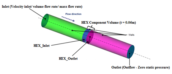
Figure 1.
Start HyperWorks CFD and Open the HyperMesh Database
-
From the Home tools, Files tool group, click the Open Model tool.

Figure 2.The Open File dialog opens.
Validate the Geometry
The Validate tool scans through the entire model, performs checks on the surfaces and solids, and flags any defects in the geometry, such as free edges, closed shells, intersections, duplicates, and slivers.
Figure 3.
Set Up Flow
Set the General Simulation Parameters
-
From the Flow ribbon, click the Physics tool.

Figure 4.The Setup dialog opens. -
Under the Physics models setting:
- Verify that Time marching is set to Steady.
- Select Spalart-Allmaras as the Turbulence model.
- Activate the Heat transfer checkbox.
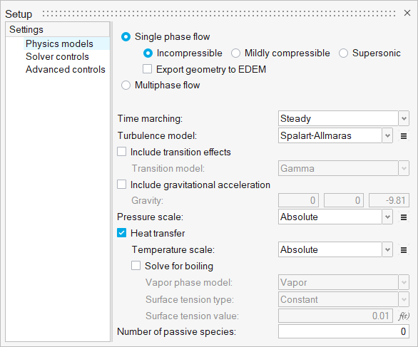
Figure 5.
Assign Material Properties
-
From the Flow ribbon, click the Material tool.

Figure 6. -
Click
 on the guide bar to exit the tool.
Define the Heat Exchanger Component
-
From the Flow ribbon, click the arrow next to the
Domain tool set, then select
Heat Exchanger.
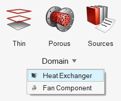
Figure 7. -
Select the middle solid as the heat exchanger component volume.
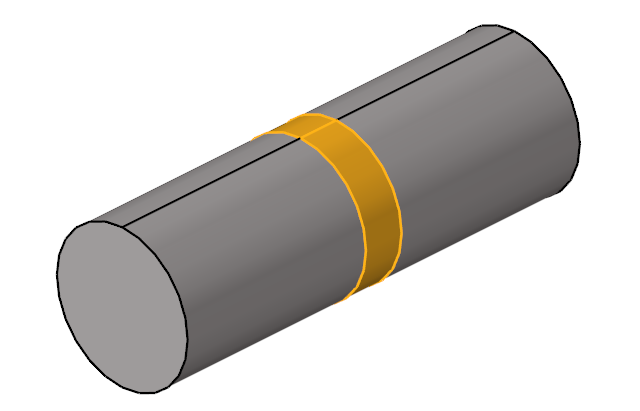
Figure 8. -
On the guide bar, click Inlet
then select the face shown below as the inlet of the heat exchanger
component.
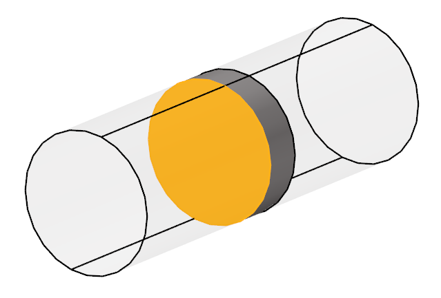
Figure 9. -
In the microdialog, enter the following
parameters:
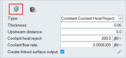
Figure 10.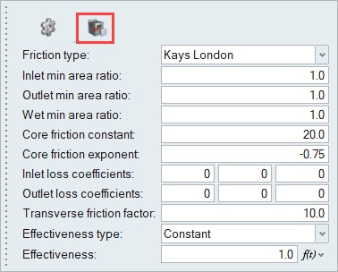
Figure 11. -
On the guide bar, click
 to execute
the command and exit the tool.
to execute
the command and exit the tool.
Define Flow Boundary Conditions
-
From the Flow ribbon, click the Constant tool.

Figure 12. -
Click the inlet face highlighted in the figure below.
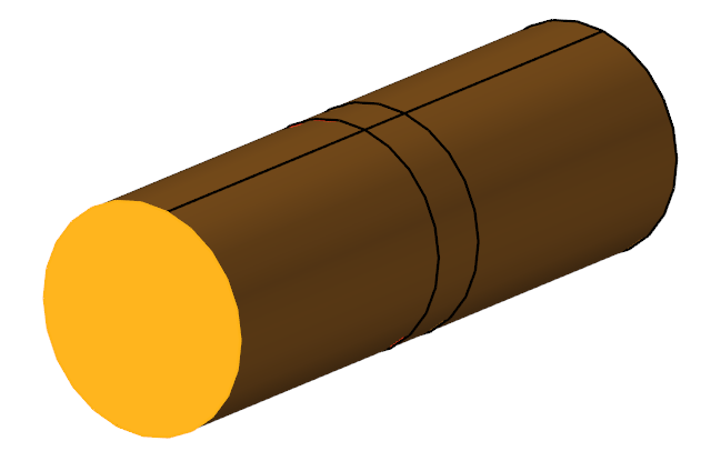
Figure 13. -
In the microdialog, enter the following values for the
Momentum and Turbulence tabs.
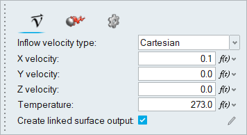
Figure 14.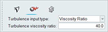
Figure 15. -
On the guide bar, click
to execute
the command and exit the tool.
-
Click the Outlet tool.

Figure 16. -
Select the face highlighted in the figure below and then click on the
guide bar.
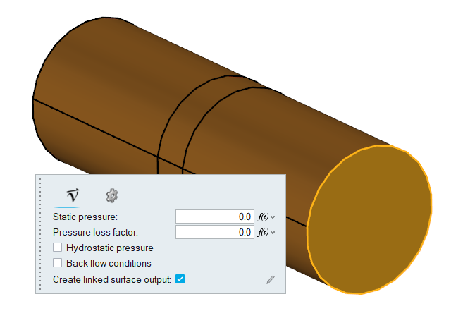
Figure 17.
Generate the Mesh
-
From the Mesh ribbon, click the
Volume tool.

Figure 18. -
In the Meshing Operations dialog, set the Mesh growth rate
to 1.1 (if not set already).
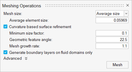
Figure 19.
Run AcuSolve
-
From the Solution ribbon, click the Run tool.

Figure 20.The Launch AcuSolve dialog opens. -
Leave the remaining options as default and click
Run to launch AcuSolve.
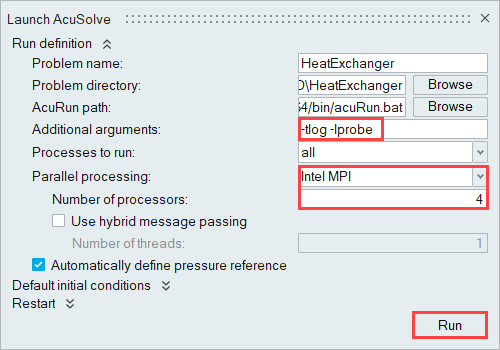
Figure 21.
Post-Process with AcuProbe
As the solution progresses, the AcuTail and AcuProbe windows are launched automatically. The surface output and residual ratios can be monitored using AcuProbe.
-
In the AcuProbe window, under the Data Tree, expand Residual Ratio,
right-click on Final, and select Plot
All.
Note: You might need to click
 on the toolbar in order to
properly display the plot.
on the toolbar in order to
properly display the plot.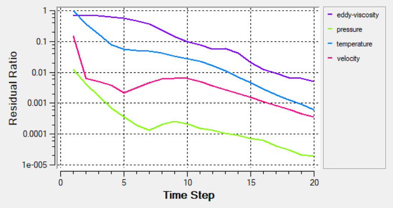
Figure 22. -
Click
 on the toolbar.
A User Function dialog opens.
on the toolbar.
A User Function dialog opens. -
On the next line, type value = Out - In.
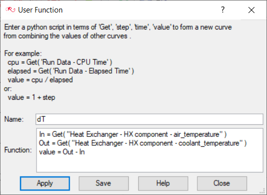
Figure 23.Note: The word “value” is case sensitive and should always be in lowercase characters. If it starts with a capital letter, it will give you an error window. -
Click Apply.
As shown in the plot below, for the given problem, the temperature rise is 43.30 K.
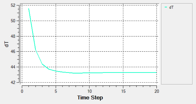
Figure 24.
Summary
In this tutorial, you successfully learned how to set up and solve a simulation involving a Heat Exchanger component using HyperWorks CFD. You started by opening the HyperMesh input file with the geometry and then defined the simulation parameters, the heat exchanger component, and the flow boundary conditions. Once the solution was computed, you defined a user-function in AcuProbe in order to create a plot of the temperature rise across the heat exchanger volume.