ACU-T: 2300 Atmospheric Boundary Layer Problem – Flow Over Building
Prerequisites
Prior to starting this tutorial, you should have already run through the introductory tutorial, ACU-T: 1000 Basic Flow Set Up. To run this simulation, you will need access to a licensed version of HyperWorks CFD and AcuSolve.
Prior to running through this tutorial, copy HyperWorksCFD_tutorial_inputs.zip from <Altair_installation_directory>\hwcfdsolvers\acusolve\win64\model_files\tutorials\AcuSolve to a local directory. Extract ACU-T2300_Building.hm from HyperWorksCFD_tutorial_inputs.zip.
Since the HyperWorks CFD database (.hm file) contains meshed geometry, this tutorial does not include steps related to geometry import and mesh generation.
Problem Description
The problem to be addressed in this tutorial is shown schematically in Figure 1. As an example, this problem shows the capability of Atmospheric Boundary Layer modelling in AcuSolve.
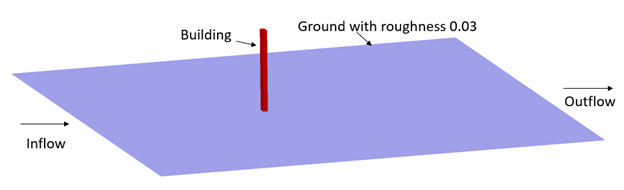
Figure 1.
In this tutorial, you will simulate the air flow over a building with a ground roughness of 0.03. In this case, User Defined Atmospheric Roughness Type is considered.
Start HyperWorks CFD and Open the HyperMesh Database
-
From the Home tools, Files tool group, click the Open Model tool.

Figure 2.The Open File dialog opens.
Validate the Geometry
The Validate tool scans through the entire model, performs checks on the surfaces and solids, and flags any defects in the geometry, such as free edges, closed shells, intersections, duplicates, and slivers.
Figure 3.
Set Up Flow
Set Up the Simulation Parameters and Solver Settings
-
From the Flow ribbon, click the Physics tool.

Figure 4.The Setup dialog opens. -
Under the Physics models setting:
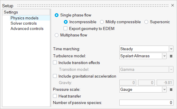
Figure 5. -
Set the Steady update factor to 0.6 and the Steady
maximum steps to 20.
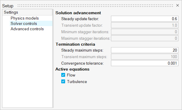
Figure 6.
Assign Material Properties
-
From the Flow ribbon, click the Material tool.

Figure 7. -
Click
 on the guide bar.
Define Flow Boundary Conditions
-
From the Flow ribbon, click the
Atmospheric tool.

Figure 8. -
Click the inlet face highlighted in the figure below.
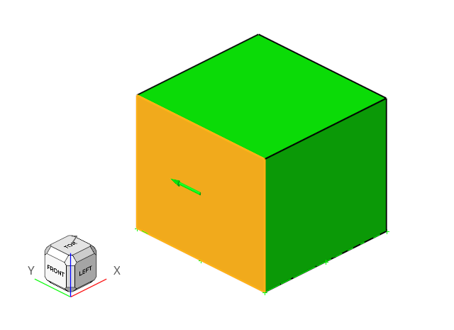
Figure 9. -
Click the Move tool icon
 .
.
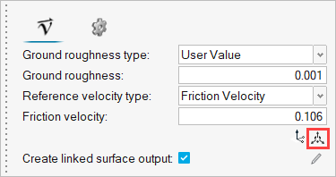
Figure 10. -
Select the z rotation arrow, set it to
-90 degrees, then press Enter.
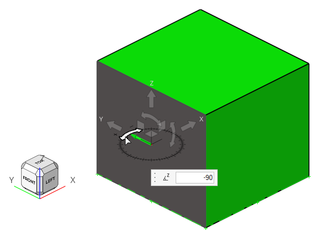
Figure 11. -
Verify the atmospheric flow direction (y) is aligned to the global coordinate
X.
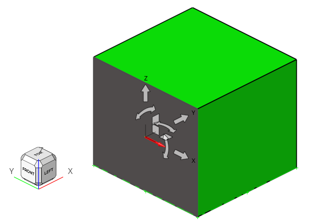
Figure 12. -
Select the y rotation arrow, set it to
-90 degrees, then press Enter.
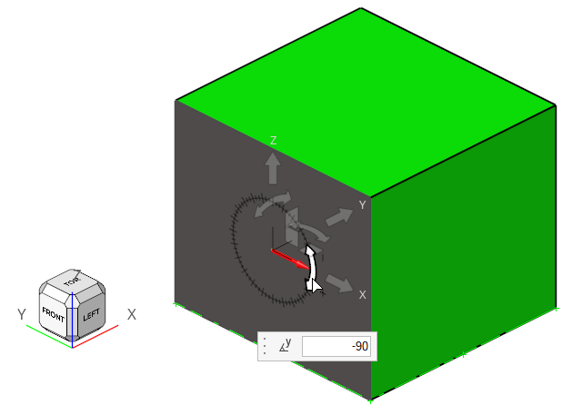
Figure 13. -
Verify the ground normal direction (x) align to the global coordinate Z.
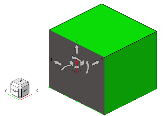
Figure 14. -
Click the origin of the coordinate (marked by the arrow), set the atmospheric
ground origin to (0, 0, 0), and press Enter.
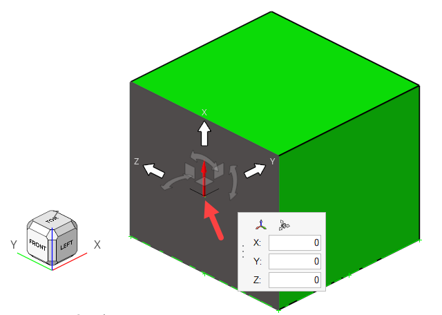
Figure 15. -
On the guide bar, click
 to execute
the command and exit the tool.
to execute
the command and exit the tool.
-
Click the Outlet tool.

Figure 16. -
Select the face highlighted in the figure below, verify that both the static
pressure and the pressure loss factor are 0 in the
microdialog, then click on the
guide bar.
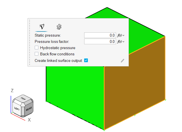
Figure 17. -
Click the Slip tool.

Figure 18. -
Select the top surface and the two sides as shown in the figure below then
click on the guide bar.
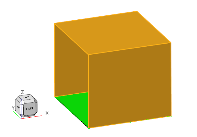
Figure 19. -
Click the No Slip tool.

Figure 20. -
Set the Roughness height to 0.03.
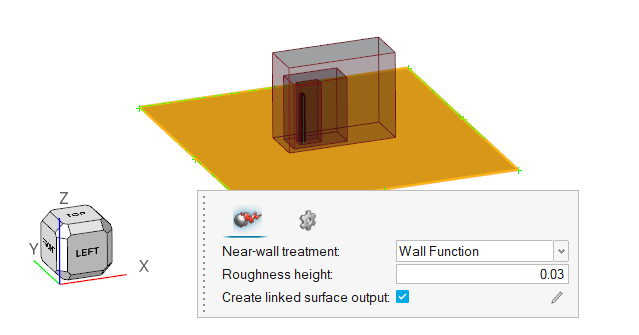
Figure 21. -
On the guide bar, click
to execute
the command and exit the tool.
Run AcuSolve
-
From the Solution ribbon, click the Run tool.

Figure 22. -
Leave the remaining options as default and click
Run to launch AcuSolve.
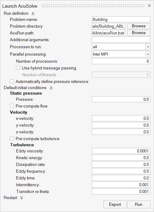
Figure 23.The Run Status dialog opens. Once the run is complete, the status is updated and you can close the dialog.Tip: While AcuSolve is running, right-click on the AcuSolve job in the Run Status dialog and select View Log File to monitor the solution process.
Post-Process the Results with HW-CFD Post
-
Click the Slice Planes tool.

Figure 24. -
Select the slice plane shown below.
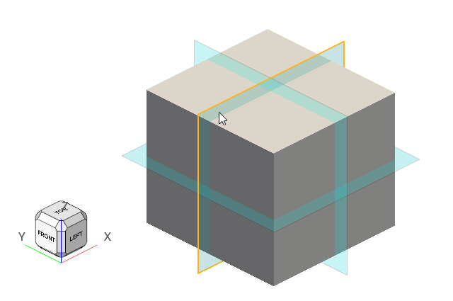
Figure 25. -
In the slice plane microdialog, click
 to
create the slice plane.
to
create the slice plane.
-
Click
 and set the Colormap name to Rainbow
Uniform.
and set the Colormap name to Rainbow
Uniform.
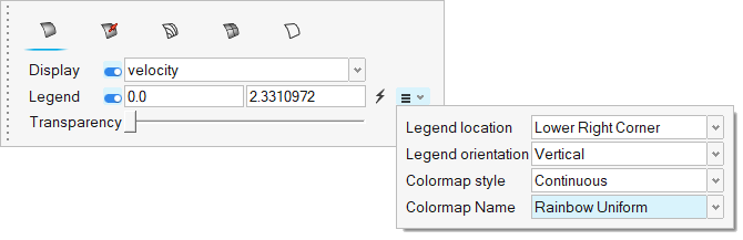
Figure 26. -
Click the Left face on the View Cube to orient the slice
plane.
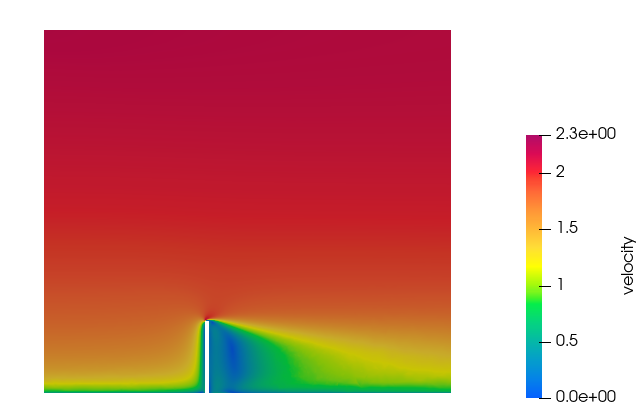
Figure 27.
Summary
In this tutorial, you successfully learned how to set up and solve a simulation involving an atmospheric boundary condition using HyperWorks CFD. You started by opening the HyperWorks CFD input file with the geometry and then defined the simulation parameters, fluid material, and boundary conditions. Once the solution was computed, you visualized the results of the velocity magnitude on a plane.