Exposable Parameters in Modelica Blocks

Exposing Parameters

You can define the values of Modelica block parameters using expressions with exposable parameters, though not all Modelica parameters can be exposed; the restrictions are similar to those of Activate block parameters, mainly that the parameters should not be structural.

Examples: Exposable parameters with Modelica blocks

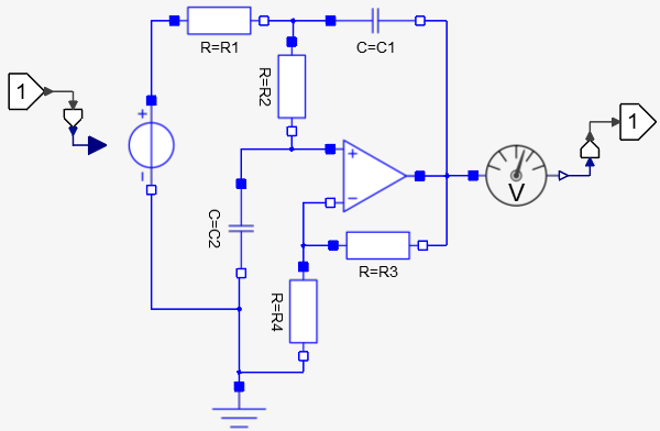
The following is a model of a Sallen-Key low-pass filter:

The filter transfer function can be expressed as follows:

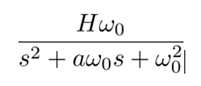
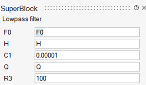
The filter is usually specified in terms of its cutoff frequency F₀ = ω₀/(2π), quality factor Q = 1/a, and gain H. These parameters will be used as exposable parameters for this model. The resistor and capacitor values should be computed as a function of these parameters.

The system of equations defining the resistor and capacitor values as functions of filter parameters is underdetermined; for example, C1 and R3 can be chosen arbitrarily, and the other values computed as follows:

This OML script is placed in the Context of the diagram containing the model of the filter. The diagram is then placed inside the Super Block in the following model:

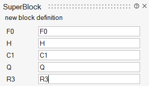
Auto-masking the Super Block determines the free parameters of the model:

Code generation can now be used; however, this would expose R3 and C1 in addition to the filter parameters. To set the values of R3 and C1 once and for all, these values can be provided numerically in the mask before applying the code generator, for example:

After the application of code generation, the following mask is generated, showing the exposed parameters:

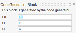
As expected, the filter parameters are exposed.

Mixing Activate and Modelica Blocks in Models

The process of defining, manipulating, and exposing parameters is similar for Activate and Modelica blocks. Indeed, what is referred to as Modelica blocks, that is Activate blocks representing Modelica components, are parameterized in the same way as “regular” Activate blocks. So, not only can Activate and Modelica blocks with exposable parameters be used in the same model, but the same exposable parameters can be used in the expressions used to define the parameter values of both types of blocks.

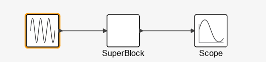
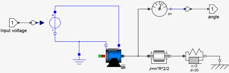
An example of an electromechanical system modeled using Modelica blocks and controlled by a discrete-time controller implemented with Activate blocks, is considered here. The electromechanical part consists of a DC motor controlled by an input voltage, rotating a mass attached to a grounded spring damper system.

The inertia of the mass is assumed to be mR²/2. The parameters m and R should be exposed.

This diagram is included in the following diagram that also contains the control action realized by a discrete transfer function.

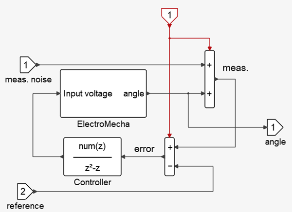
The denominator of the transfer function is fixed (chosen to obtain infinite gain at zero frequency to reject constant bias); the numerator (vector) is the control parameter, which should be exposed. The controller input is the difference between the measured angle and a reference angle. The measured angle is obtained by sampling the actual output and adding measurement noise.

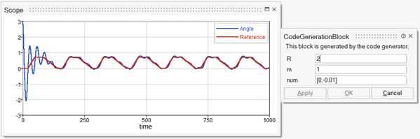
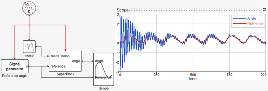
You can see the complete model in the following diagram where the measurement noise and the reference angle are provided. A Scope plots the actual angle and the reference angle. The frequency of the sampling is set to 10Hz. The parameter values are m=1, R=2 and num= [-0.1,0.04].

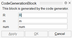
Applying code generation to the block exposes the parameters as expected:

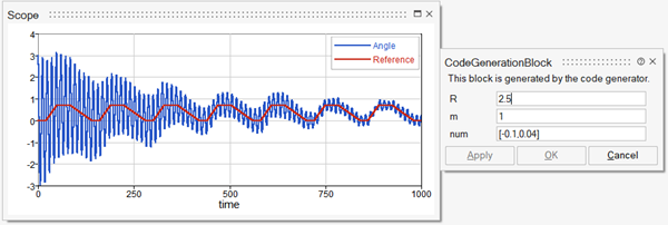
You can now perform simulations with different parameter values by providing new values in the mask. For example, the robustness can be examined by changing the value of R:

Similarly, the values of m and num can be modified. Note however that the length of num must be 2 and cannot be changed as exposable parameter sizes are fixed. In the case of the transfer function blocks in particular, the length of the numerator vector must one less than the degree of the denominator. So, for example if the transfer function -0.01/(z²-z) is desired, then the value of the num parameter should be set to [0,-0.01], instead of the usual [-0.01]: