Delay Process
The Delay Process is a post-process computation that shows how a given signal is distorted in the time domain because of its environment. The signal, which may be set with different shapes, is generated by every antenna source available in the simulation, and the delay process may be computed in multiple near field observation points.
After running a Delay Process type simulation, click on View Delay Process to open the Delay Process window, and the following panel is shown on the right side:
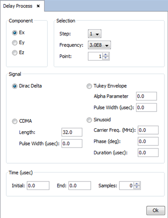
Figure 1. Delay process configuration panel
This panel contains several options for plotting the Delay Process:
- Component: specify the component considered for the Delay Process computation (Ex, Ey or Ez).
- Selection to define the spherical far-field ranges where the
Delay Process will be computed. The first row defines the
theta interval and the second row the phi one.
- Step select the step of the parametric simulation to be consider. If it is not a parametric simulation, this value will be 1.
- Frequency frequency of the simulation.
- Point select the observation point index to consider in the Delay Process.
- Signal the original signal may be generated by using different
patterns. All of them are configured in the time domain.
- Dirac Delta only a pulse is generated in the initial time.
- CDMA a random distribution of pulses centred with positive (high) an negative (low) levels is generated. Note that a low or high level is considered as a Pulse.
-
- Length number of pulses to be generated.
- Pulse Width time duration of each Pulse, in microseconds.
- Sinusoid a sinusoidal signal is generated.
-
- Carrier Freq. frequency of the sinusoidal signal, in MHz.
- Phase initial phase of the sinusoidal signal, in degrees.
- Duration total length of the generated sinusoid in the time domain, in microseconds.
- Tukey Envelope a Gaussian signal enveloped by a rectangular pulse is generated.
-
- Alpha Parameter define the slope of the Gaussian curve. The higher is this parameter, the more enveloped by the rectangular pulse is the generated signal.
- Pulse Width define the total length of the generated signal in the time domain, in microseconds.
- Time this section specifies the observation time range.
-
- Initial
- first observation instant in the time domain, in microseconds.
- End
- last observation instant in the time domain, in microseconds.
- Samples
- number of instants to evaluate deDelay Processthat are equally equispaced in the time domain.
Click on OK button to plot de Delay Process results.
Only when the CDMA signal has been selected, the window represented below aks the selection of the Correlation Signal to be plotted with the following options.
- Input (x[n]) the original CDMA signal is represented.
- Output (y[n]) the received CDMA signal is represented Correlation (c[n]) the correlation on the received signal is represented.
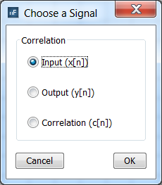
Figure 2. Selection of signal to be plotted with CDMA
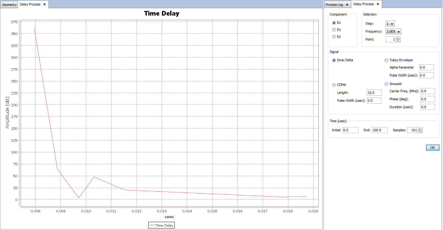
Figure 3. Delay Process generated with a Dirac Delta signal
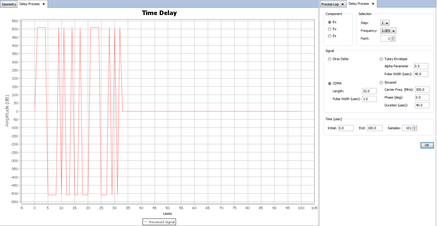
Figure 4. Delay Process generated with a CDMA (output y[n]) signal
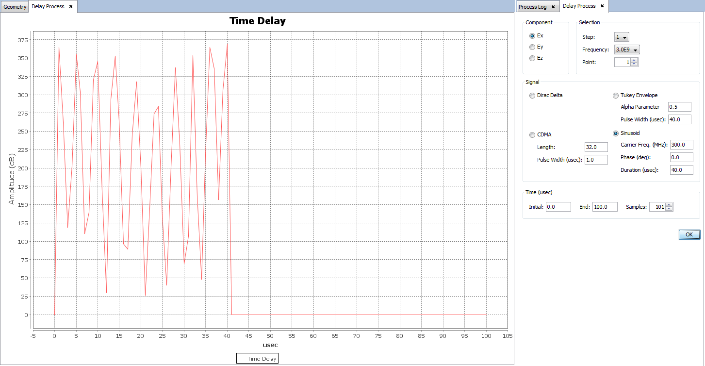
Figure 5. Delay Process generated with a Sinusoid signal
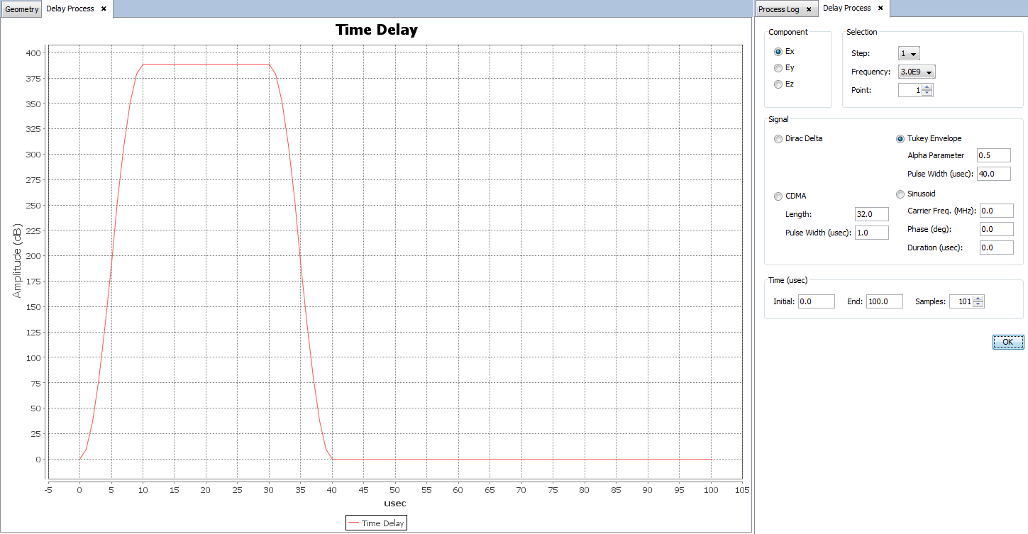
Figure 6. Delay Process generated with a Tukey Envelope signal