Calculate propagation between a static transmitter and a moving car in a suburban
scenario.
Model Type
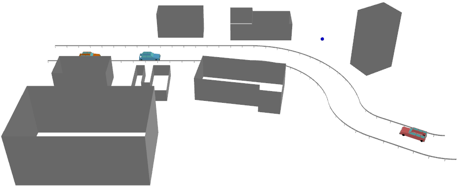
The propagation between a static transmitter at a height of 3 m next to the road with
a moving car is calculated.
Sites and Antennas
The transmitting antenna is an omnidirectional antenna at 2 GHz. The database for
this time-dependent moving car is defined in WallMan.
The transmitter is located beside the road.
Figure 1. Model of the suburban structures and topography.
Computational Method
This project uses a semi-deterministic prediction model, dominant path model (DPM), to compute the power distribution in the area.
Tip: Click Project > Edit Project Parameter and click the Computation tab to change
the model.
This model does not compute multipath propagation, but only the dominant path to each
receiver location. For large scenarios, this computation method takes less time than
compared to a ray-optical computation method.
Results
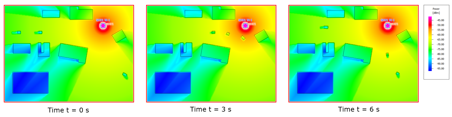
The results are computed for six time stamps in this model, from 0 s to 6 s in steps
of 1 s. The received signal power is displayed for three different timestamps, see
Figure 2.
Figure 2. Received signal power for three different timestamps.