3D Intelligent Ray Tracing
This model performs a rigorous 3D ray-tracing prediction which results in a high accuracy and with the pre-processing of the database, the computation time is short.
The mobile radio channel in urban areas is characterized by multi-path propagation. Dominant propagation phenomena in such built-up environments are the shadowing behind obstacles, the reflection at building walls, wave guiding effects in street canyons and diffractions at vertical or horizontal wedges. The deterministic ray optical models consider these effects, which leads to accurate prediction results.
- The deterministic modeling of path finding generates a large number of rays, but only few of them deliver the main part of the received electromagnetic energy.
- The visibility relations between walls and edges are independent of the position of the base station.
- In many cases neighboring receiving points are hit by rays whose paths differ only slightly. For example, every receiving point in a street orthogonal to the street in which the transmitter is located and it is hit by a double reflected - single vertically diffracted ray and the points of interaction of these rays with walls and edges are independent of the receiver position.
Based on these considerations it is possible to accelerate the time consuming process of ray path finding by a single intelligent pre-processing of the data base for buildings.
Principle
The intelligent ray-tracing technique allows it to combine the accuracy of ray optical models with the speed of empirical models. To achieve this, the database undergoes a sophisticated pre-processing. In a first step the walls and edges of the buildings are divided into tiles and segments, respectively. Horizontal and vertical edge segments are distinguished. For every determined tile and segment all visible elements (prediction pixels, tiles and segments) are computed and stored in file.
For the determination of the visibility the corresponding elements are represented by their centers. Additionally, the occurring distances as well as the incident angles are determined and stored. Due to this pre-processing the computational demand for a prediction is reduced to the search in a tree structure. The following picture shows an example of a tree consisting out of visibility relations.
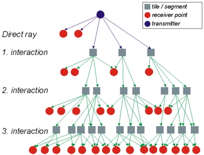
Figure 1. Tree of visibility relations.
Only for the base station with an arbitrary position and antenna pattern (not fixed at the pre-processing), the visible elements including the incident angles have to be determined at the prediction. Then, starting from the transmitter point, all visible tiles and segments are tracked in the created tree structure considering the angle conditions. This tracking is done until a prediction point is reached or a maximum number of interactions (reflections / diffractions / transmissions (only indoor) ) is exceeded. The following picture shows the division into tiles and segments.
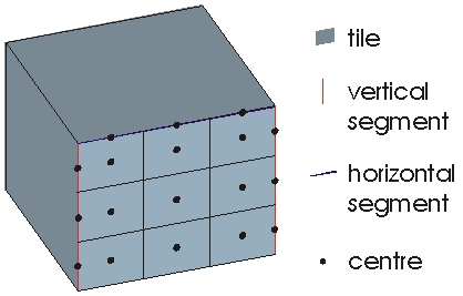
Figure 2. Division into tiles and segments.
The following picture shows an example of a ray path between a transmitter and a receiver with a single reflection. The tiles and segments are also visible. These are examples of an urban database. The procedure with indoor databases is the same, only transmissions are additionally considered.
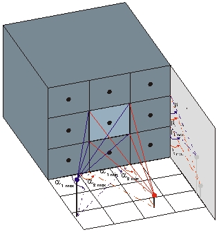
Figure 3. Example of a ray path between a transmitter and receiver with a single reflection.
- 2x2D (2D-H IRT + 2D-V IRT)
- The pre-processing and as a follow on also the determination of propagation paths is done in two perpendicular planes. One horizontal plane (for the wave guiding, including the vertical wedges) and one vertical plane (for the over rooftop propagation including the horizontal edges). In both planes the propagation paths are determined similar to the 3D-IRT by using ray optical methods.
- 2x2D (2D-H IRT + COST231-W-I):
- This model treats the propagation in the horizontal plane in exactly the same way as the previously described model by using ray optical methods (for the wave guiding, including the vertical wedges). The over rooftop propagation (vertical plane) is taken into account by evaluating the COST 231-Walfisch-Ikegami model.
The pre-processing is not done within ProMan but has to be done within the WallMan application.
Settings
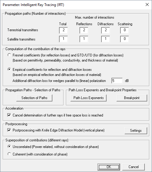
Figure 4. The Parameter: Intelligent Ray Tracing (IRT) dialog.
- Propagation paths (number of interactions
- This dialog allows to specify how many interactions should be considered for the determination of ray paths between transmitter and receiver including maximum number of reflections, diffractions and scattering. Separate definitions for terrestrial and for satellite transmitters are possible.
- Computation of the contribution of the rays
- The deterministic mode uses Fresnel equations for the determination of the reflection and transmission loss and the GTD / UTD for the determination of the diffraction loss. This model has a slightly longer computation time and uses four physical material parameters (thickness, permittivity, permeability and conductivity). In case of a full polarimetric analysis, the deterministic mode should be selected. In case of a standard analysis, it is optional.
The empirical mode uses five empirical material parameters (minimum loss of incident ray, maximum loss of incident ray, loss of diffracted ray, reflection loss, transmission loss). For correction purposes or for the adaptation to measurements, an offset to those material parameters can be specified.
The empirical model has the advantage that the needed material properties are easier to obtain than the physical parameters required for the deterministic model. Also, the parameters of the empirical model can be calibrated with measurements more easily.
The diffraction loss depends besides the angles of the given propagation path also on the relationship between the wedge direction and the polarization direction. According to physics and verified by measurements there is an additional loss of about 5 dB if both directions are parallel (for example, diffraction on vertical wedge for vertically polarized signal). While this effect is automatically considered if using the GTD / UTD model, a corresponding offset is available for the empirical diffraction model. This additional loss is added to the diffraction loss in case the wedge direction and the polarization direction are parallel. In case the wedge direction and the polarization direction are orthogonal no additional loss is considered. In between there is a linear scaling of this additional loss.
Diffuse scattering in urban scenarios can play an important role, especially for determining the actual temporal and angular dispersion of the radio channel. The IRT model for urban scenarios has been extended to consider the scattering on building walls and other objects. For this purpose the scattering can be activated in the model settings (where also the number of reflections and diffractions are defined). As the scattering increases the overall number of rays significantly, there is a limitation of one scattering per ray. The single scattering is considered as separate ray and also in combination with other interactions (transmission, reflection and diffraction).
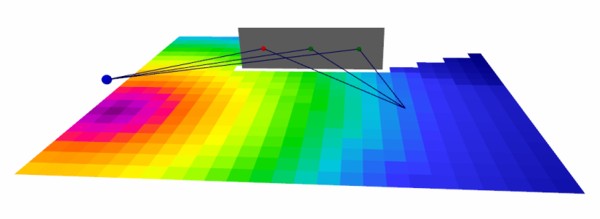
Figure 5. Example of diffuse scattering.
Furthermore, the scattering properties of the corresponding materials need to be defined (in WallMan and ProMan). Both the empirical and the deterministic (physical) interaction models are supported. In the empirical interaction model the scattering loss defines the additional loss (for a ray 30° out of the reflection direction). The scattering loss is added to the reflection loss. The defined scattering loss is applied if the angle difference between reflected and scattered ray is 30°. In case of 0° no additional scattering loss is applied.
Generally, the scattering loss is increasing with increasing angular difference. In the deterministic model the polarimetric scattering matrix , , , is defined and considered for the field strength computation. For the scattering in the IRT model the tiles as defined in the WallMan pre-processing are considered. The scattered contribution is weighted with the size of the scattering area (tile) with a reference size of 100 sqm.
- Propagation Paths (Selection of Paths)
- Limitation of number of paths per pixel with the following options:
- maximum path loss of rays
- maximum number of paths
- dynamic range of paths
- Consideration of Rays for Computation of Angular Spread and Mean
- During computation of delay or angular spread and mean, the contribution of each propagation path to the delay or angular spread/mean is considered. Each path contributes a signal level to the spread. This level can be either considered as power (in dBm or Watt) or as field strength (in dBµV/m or in µV/m). Power values include the gain of the Rx antenna and depend on the frequency, whereas field strength values do not depend on the frequency. The values can be considered either in logarithmic scale (dBm or dBµV/m) or in linear scale (mW or µV/m).
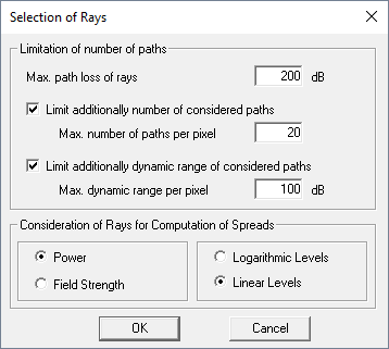
Figure 6. The Selection of Rays dialog.
- Path Loss Exponents and Breakpoint Properties
-
The breakpoint describes the physical phenomenon that from a certain distance on the received power decreases with 40 log(distance/km) instead of 20 log(distance/km) which is valid for the free space propagation. This is due to the superposition of the direct ray with a ground reflected contribution.
Exponent before breakpoint (LOS/NLOS) / Exponent after breakpoint (LOS/NLOS). These four exponents influence the calculation of the distance dependent attenuation. For further refined modeling approaches different exponents for LOS and NLOS conditions can be applied. The default values are 2.4 and 2.8 for the exponents before the breakpoint (LOS and NLOS) and 3.6 and 4.0 for the exponents after the breakpoint (LOS and NLOS).
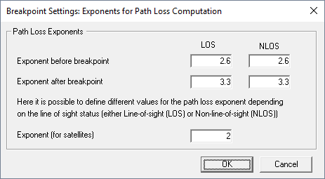
Figure 7. The Breakpoint Settings dialog.
The breakpoint distance depends on the height of transmitter and receiver as well as the wavelength. The initial value is calculated according to . This value can be modified by setting an additional offset (in meters).
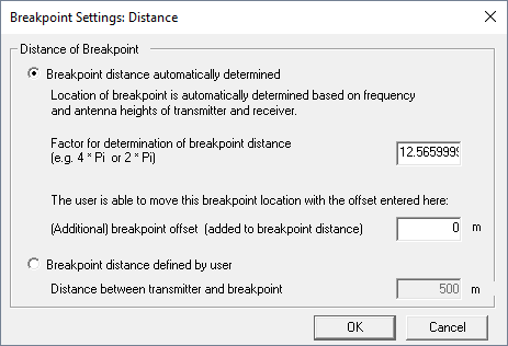
Figure 8. The Breakpoint Settings dialog.
- Acceleration
-
Further options exist to accelerate the prediction model. If many rays are received at a pixel, the sum of the contributions of all rays might be higher than the contribution of the LOS ray to this pixel. Then you can decide to stop the computation for this pixel and no further rays are determined to save computation time.
But it makes only sense if you look at the signal level, because if you have already achieved -80 dBm at the pixel with a few rays, a further ray with -95 dBm does not modify the total power for this pixel.
You can even add 5 rays with -95 dBm each to this pixel - the total power will remain at -80 dBm. So it makes actually sense to ignore all further rays as they have nearly no impact on the predicted power result. But when you want to compute the delay spread or angular spread, you need obviously all rays to get an accurate result.
If you have one ray with 80 dBm and 5 further rays with -95 dBm each, the signal level might be -80 dBm if you consider 1 ray or 6 rays. But the delay spread would be 0 ns in case of one ray and 5 ns or 10 ns or 15 ns if you consider all 6 rays. So you cannot neglect further rays if you are predicting the delay spread or the angular spread.
- Post Processing
- [Optional] Prediction results can be post processed using the knife-edge diffraction model. Parameters for this model can be specified on a separate dialog which can be found by clicking Settings.