BasicFEA-1000: Run a Linear Static Analysis

In this tutorial, you will learn to:

•	Run a simple linear static analysis. The default solver used is OptiStuct.

This exercise uses the Full_Motion_TV_Mount_Partly_Open.hm file, which can be found in the hm.zip file. Copy the file(s) from this directory to your working directory.

1.	Launch HyperMesh. The User Profiles dialog opens.

2.	Select BasicFEA from the Application drop-down and click OK or click Preferences > User Profiles to open the dialog.

Note:

You can also launch BasicFEA from the Start menu by clicking All Programs > Altair HyperWorks <version > BasicFEA.

1.	Copy the model provided for linear static analysis into a directory on your computer.

2.	Right-click anywhere in the BasicFEA browser. This opens a context menu that contains several relevant functions.

3.	Click Open to display a dialog that allows you to load the model.

Browse to the directory on your computer where the model is stored and load the model by selecting it and clicking Open. The model used for this tutorial is Full_Motion_TV_Mount_Partly_Open.hm. This model does not contain any other information except geometry information and units metadata. BasicFEA organizes and creates properties and materials upon import.

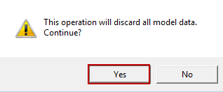
Note:

When you load the model into BasicFEA all existing model data is deleted and replaced.

fea_1000_discard_data

Note:

Pressing CTRL on the keyboard while clicking the model allows you to zoom in and out.

1.	After the model is loaded, the wireframe geometry of the model displays. To view the model better and to get a feel for the way it looks after fabrication, click the icon in the BasicFEA toolbar.

2.	Right-click Mode: Geometry in the BasicFEA browser and select Mesh to view the default mesh on the model. BasicFEA generates a default mesh for the model without the need for you to do anything.

fea_1000_meshed_model

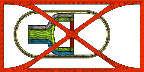
Meshed model

3.	The model is changed back to Geometry for the rest of the analysis setup.

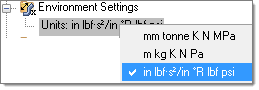
4.	The units of the model are set up by default, but you can change them by right-clicking Units in the BasicFEA browser. For this exercise the English FPS system is used (in Ibf-s^2/in *R Ibf psi).

fea_units

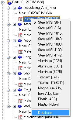
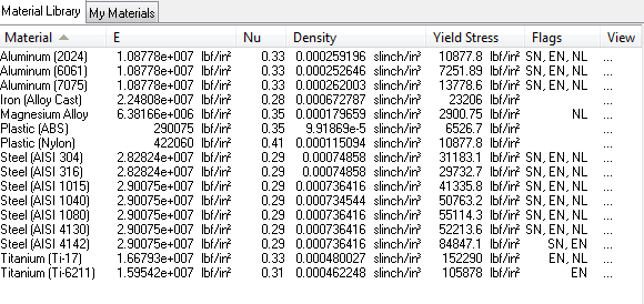
5.	Materials are assigned by default for each part. Right-clicking a part and selecting Material provides a list that contains the commonly used materials. Clicking Database opens a Material Database dialog with the complete database of all available materials.

fea_1000_material

fea_1000_material_database

6.	Click the My Materials tab and the plus icon to add a new user defined material to the database.

material_database_dialog

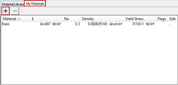
7.	Name the new material Basic and change the Young's Modulus (E) to 3.0 e 07 and the Poisson's ratio (Nu) to 0.3.

8.	Close the Material Database dialog.

9.	After the new material is added, right-click Material underneath any of the parts and select Basic from the list of materials. The name of the material now shows.

fea_1000_material_basic

10.	The dimensions of the model can be checked by clicking the icon in the BasicFEA toolbar. This step is optional.

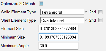
11.	If the default model settings are not satisfactory you can change them by right-clicking a part and selecting Mesh Settings. This opens the Mesh Settings dialog. This step is optional.

fea_1000_mesh_settings

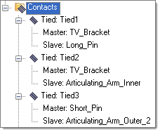
Since the model consists of different parts, they have to be connected before analysis. The simplest form of connection is a tied contact between touching parts.

1.	Right-click Contacts in the BasicFEA browser and select Create> Auto-contact. Auto contact will search the model for touching parts and create a tied contact between each of them.

fea_1000_contact

1.	As you have seen in the previous steps, the right-click context menu is used to create a new linear static loadstep. Right-click Loadsteps in the BasicFEA browser and select Create > Linear Static Loadstep.

2.	After the loadstep is added the loads and constraints need to be created on the model. Right-click Linear Static Loadstep > Create Constraint > On Surface.

3.	Select the surface where the constraints need to be applied.

4.	After selecting the surface, click proceed to create the constraints. The model view is changed to wireframe to view the constraints. The view can be changed back to shared geometry and surface edges after looking at the constraints.

5.	Right-click Constraint > Translation to change the nature of the assigned constraints. This option locks the translation movement of the selected surface in all three directions (X, Y, Z).

6.	Right-click Linear Static and select Create Total Load > On Surface.

7.	Select the surface shown in white in the image below and click proceed.

fea_1000_constraints_applied

Selecting the surface on which constraints are applied

tv_stand

Selecting the surface for the application of distributed loads

To change the nature of the applied load, click the magnitude next to Total Load. Make sure the load is highlighted before clicking the value to edit it. For this example a magnitude of -2.98 is assigned to the total load. The direction of the total load is set by right-clicking Total Load > Direction> Global Y.

9.	In the BasicFEA browser right-click and select Save as to save the model before analysis. Select any location you prefer to save the model and save it as a HyperMesh (.hm) file.

Note:

The surfaces for which you want to apply constraints or loads turn white in color as you click them. This makes it easier for you to distinguish them from the other surfaces.

1.	Click the icon in the BasicFEA toolbar to run the analysis. The HyperWorks Solver View dialog opens, allowing you to see the progression of the analysis.

After the completion of the job the dialog can be closed to view the results of the analysis in HyperMesh. The Contour panel is automatically loaded, and a contour plot can be viewed in HyperMesh by selecting the desired type of output from the Contour panel options. The simulation and data type options control the requested plots and the contour and assign buttons apply the result to the nodes and elements. It is best to use assign with elements results like stresses, and contour with nodal results like displacements.

Note:

There are other methods to review the Results under the right-click context menu. Select Contour plot to display a colored static plot as described above. Select Vector plot to animate or show the deformed shape. The deform button shows the deformed shape, and the linear and modal buttons run the animation.