Viewing the Results
View and post-process the results in POSTFEKO.
-
Create the input Gaussian pulse and triangular pulse using the following
parameters:
Property Gaussian pulse Triangular pulse Time axis unit ns ns Total signal duration 100 100 Amplitude 1 1 Pulse delay 19 19 Pulse width 4 8 Number of samples 400 400 Tip: On the Time analysis tab, in the Time signal group, click the New time signal icon.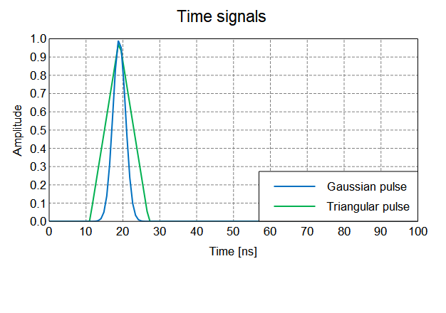
Figure 1. The Gaussian and triangular input signals. -
View the time response of the system when a Gaussian pulse or a triangular
pulse is applied.
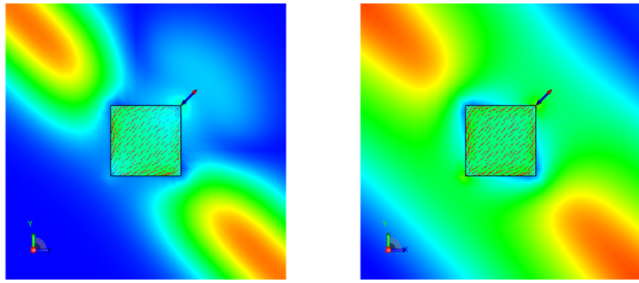
Figure 2. Near field time response for the Gaussian pulse (left) and triangular pulse (right) after 19 ns.Note: Gain insight into the time domain behaviour of a system using animation. -
View the near field magnitude plotted over time at position (-2, -2, 0)
m.
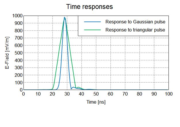
Figure 3. E-field magnitude at position (-2, -2, 0) m.