
To perform a Nyquist stability analysis, consider a simple type 0 system with the open-loop transfer function:
as shown in the diagram below.
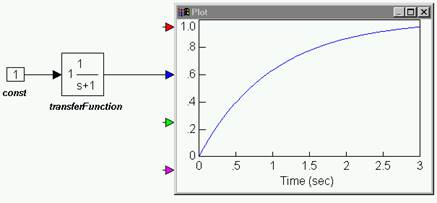
To generate the Nyquist plot
1. Create the above diagram using a const, transferFunction, and plot block.
2. Enter the following polynomial coefficients to the transferFunction block:
Numerator: 1
Denominator: 1 1
Note: Always leave spaces between coefficient values.
3.
Choose System > Go, or click  in the toolbar to simulate the diagram.
4. Select the transferFunction block.
5. Choose Analyze > Nyquist Response.
The Nyquist plot is displayed.
6. Drag on its borders to adjust its size.
The Nyquist plot for this system is a circle, with the real part of GH(s) on the horizontal axis and the imaginary part of GH(s) on the vertical axis. On this plot, the origin represents GH(j∞) and the point of intersection with the horizontal axis (Re(GH) = 1) represents GH(j0).