Block Category: Integration
Input: Real scalar
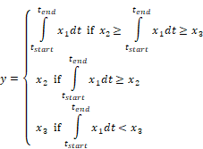
Description: The limitedIntegrator block integrates the input value and limits the internal state to specified upper and lower limits. If the integral state reaches its limit, it backs off the limit as soon as the derivative changes sign. You set the integration algorithm with the System > System Properties command. Available algorithms are Euler, trapezoidal, Runge Kutta 2nd and 4th orders, adaptive Runge Kutta 5th order, adaptive Bulirsh-Stoer, and backward Euler (Stiff). You can reset the integrator block to 0 using the System > Reset States command.
The inputs to the block are x1, the derivative; x2 (U), the upper limit; and x3 (L), the lower limit.
The limitedIntegrator block is used in the prevention of wind-up in PI and PID controllers in control applications. It is also used in kinematics, electrical circuits, process control, and fluid dynamics.
Code Generation: When generating code for C2000 or ARM Cortex targets and you include one or more limitedIntegrator blocks in your diagram and you activate Check for Performance Issues in the Code Generation dialog box, Embed warns you that large RAM blocks are not supported for the target. You can continue with code generation; however, the generated code may not fit in the target RAM and the code will run slower.
When generating code for Arduino or MSP430 targets, you cannot include limitedIntegrator blocks in your diagram. Embed halts code generation and issues a message to replace the block.
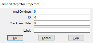
Checkpoint State: Contains the value of the integrator state at the checkpoint. If you have not checkpointed your simulation using the System > System Properties command, the value is 0. You can enter a value as a C expression.
ID: Represents an identification number for the block, which holds the state number that Embed assigns to the integrator. The number of states in any block diagram equals the number of integrators. The default is 0.
Initial Condition: Indicates the initial value of the integrator. The default is 0. You can enter a value as a C expression.
Label: Indicates a user-defined block label that appears when View > Block Labels is activated.
1. Integration with constant limits
Consider a system whose dynamics are given by the differential equation:

Furthermore, assume that x must lie in the limits 5 ≤ x ≤ 6 and that x(0) = 5. This system can be realized as shown below.
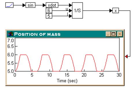
During simulation, the limitedIntegrator block limits the output to be within the upper and lower limits, namely 6 and 5, respectively.
2. Integration with time-varying limits
Consider a system whose dynamics are given by the differential equation:

Furthermore, assume that x must lie in the limits 0.2t ≤ x ≤ 2t and that x(0) = 0. This system can be realized as:
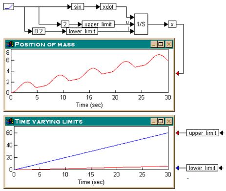
A ramp block is used to access simulation time, t; simulation time is then used to feed the sin block, and two gain blocks, set to 2 and 0.2, to generate the time-varying upper and lower limits. During simulation, the time-varying limits and the output of the limitedIntegrator block are displayed in the plot blocks.