Block Category: Matrix Operation
Inputs: Scalar
Description: The buffer block places a sequence of values in a buffer based on the buffer length, the time between successive samples, and the duration of the simulation. The buffer produces a single vector output.
When the buffer block is added to a feedback loop, the buffer updates on its dt value.
This block is useful for performing basic digital signal processing operations.
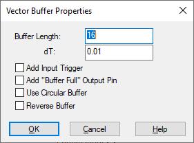
Add “Buffer Full” Output Pin: Adds an output pin that goes high when the buffer is full.
Add Input Trigger: Runs if trigger input is true (1); or does nothing if false (0).
Buffer Length: Determines the number of samples; that is, the size of the buffer.
dT: Determines the time between successive samples; that is, the rate at which samples of the incoming signal are collected and placed in the buffer. When a buffer block is added to a feedback loop, the buffer updates on its dt value.
Reverse Buffer: Reverses the order of elements in the buffer. Instead of newest to oldest they are ordered oldest to newest.
Use Circular Buffer: When activated, the buffer block performs full buffer chunks at a time. It starts writing at the far end of the buffer and finishes at the first element. If you also activated Add “Buffer Full” Output Pin, a flag is set indicating the buffer is ready.
1. Basic buffer operation
Consider the following buffer block, with a buffer length of 4 and time between successive samples of 0.01.

For simplicity, let the simulation step size be equal to 0.01. If the input to the buffer is an arbitrary non-zero signal, such as a ramp signal, then after two simulation time steps, the output of buffer is a vector of length 4, with the first two elements containing non-zero values and the remaining two still at zero. At the very next time step, the simulation appears as:

The previous values are pushed down the vector by one cell, and the top cell is occupied by the latest sample. Once the simulation goes beyond four time steps, the output will be a full vector.
Obviously, if the input signal itself is zero for some points, those values will be reflected accurately in the output.
2. Computation of FFT and inverse FFT
Consider a simple example, where a sinusoidal signal is converted to frequency domain via FFT, and then reconstructed using the IFFT.
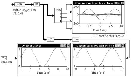
A sinusoid block generates a sinusoid signal with a frequency of 1 rad/sec. The signal is passed through a buffer block of length 128 samples and a time between successive samples of 0.01. The output of the buffer block is connected to an fft block, which computes a 128-sample FFT of the original sinusoid at a sampling rate of 0.01.
The output of the fft block is Fourier coefficients. The individual coefficients are accessed using a vecToScalar block. The first four coefficients are plotted to show their variation with time.
Signal reconstruction is performed by feeding the output of the fft block to an ifft block to compute the IFFT. The output of the ifft block is a vector of length 128 samples. The contents of this vector are just 128 sinusoid reconstructions, with each sinusoid trailing the preceding sinusoid by an amount equal to the sampling rate.
The first element in the ifft output vector does not have any delay because zero time has elapsed between the FFT and IFFT phases. In most real-world situations, however, there is a small, non-zero delay between the input signal and its reconstruction that is introduced by the processor performing the numerical computations of FFT and IFFT algorithms.