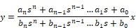
The transferFunction block executes a single-input single-output linear transfer function specified in the following ways:
•As an M file created with Embed: The Linearize command in the Analyze menu generates ABCD state-space matrices from the nonlinear system by numerically evaluating the matrix perturbation equations at the time the simulation was halted.
•As an M file created with a text editor: The following is an example of a user-written M file:
function [a,b,c,d] =vabcd
a = [-.396175 -1.17336 ; 5.39707 .145023 ];
b = [-.331182 ; -1.08363 ];
c = [0 1 ];
d = [0 ];
•As a MAT file created with MATLAB: Generating MAT files is described in the MATLAB documentation. Note that when you save the ABCD matrices to file, the names of the matrices are not important; however, the order in which they appear is.
When you simulate the block diagram, Embed numerically solves the transferFunction block.
You can set initial conditions for transferFunction blocks using variables. You can also reset transferFunction blocks to zeros using the System > Reset States command.
Digital filter design: The transferFunction block supports IIR and FIR digital filter design.
Setting up a transfer function: The transferFunction block’s Properties dialog box allows you to control how the numerator and denominator polynomials are entered.
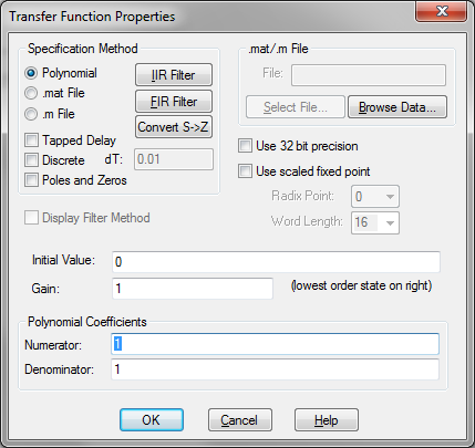
Display Filter Method: Displays the filter specification on the block. When Display Filter Method is not activated, Embed displays the polynomial coefficients.
Gain: Indicates the transfer function gain. If the leading terms of the numerator and denominator coefficients are not unity, Embed will adjust the gain to make it so. The default value is 1.
Initial Value: Specifies initial values for the states in the block. The values are right-adjusted. The right-most value corresponds to the lowest order state. Unspecified states are set to zero.
.mat/.m File: Indicates the name of the M or MAT file to be used as input to the transferFunction block. You can type the file name directly into this box or select one using the Select File button.
Denominator: Indicates the denominator polynomial for the transferFunction block. Embed determines the order of the transfer function by the number of denominator coefficients you enter. For example, an nth order transfer function will have n + 1 coefficients. Separate coefficients with spaces.
Numerator: Indicates the numerator polynomial for the transferFunction block. Separate coefficients with spaces.
Radix Point: Sets the binary point. This option can be used only when Use Scaled Fixed Point is activated.
Discrete: Indicates a discrete Z-Domain transfer function. Enter the time step for the discrete transfer function in the dT box. By default, Embed uses the step size established with the System > System Properties command. When Discrete is de-activated, a continuous transfer function is created.
dT: Specifies the time step for the discrete transfer function. By default, Embed uses step size parameter from the System > System Properties command.
.mat File: Indicates that the transfer function is to be specified as a MAT file. Specify the name of the MAT file in the .mat/.m File group box.
.m File: Indicates that the transfer function is to be specified as an M file. Specify the name of the M file in the .mat/.m File group box.
Poles and Zeros: Lets you enter a transfer function via zeros and poles in the Numerator and Denominator boxes, respectively. Enter each root in the following format:
(real-part, imaginary-part)
For large order systems, poles and zeros is more numerically accurate.
Polynomial Coefficient: Indicates that the transfer function is to be specified as numerator and denominator polynomials. Supply the numerator and denominator polynomials and gain under the Polynomial Coefficients group box.
Tapped Delay: Provides tapped delay implementation for high order FIR filters.
IIR Filter button: Opens the IIR Filters Setup dialog box to design a suitable filter using analog prototypes.
FIR Filter button: Opens the FIR Filter Setup dialog box to construct Regular Finite Impulse Response filters, differentiators, and Hilbert Transformers.
Convert S ->Z button: Uses bilinear transformation to convert a continuous transfer function to an equivalent discrete transfer function with a sampling interval of dT. Embed requests a discrete sampling rate prior to performing the conversion.
An example of the conversion is shown below.

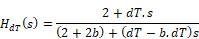
The bilinear transformation can be implemented by the substitution:

The above transfer function becomes:

Embed automatically simplifies this representation and enters the appropriate coefficients for the numerator and denominator polynomials.
Convert Z ->S button: Uses bilinear transformation to convert a discrete transfer function to an equivalent continuous transfer function. For example, consider:

The bilinear transformation can be implemented by the substitution:

The above discrete transfer function becomes:
Embed automatically simplifies this representation and enters the appropriate coefficients for the numerator and denominator polynomials.
It is important to note that in both transformations, the results obtained are dependent on the sampling interval dT. In other words, for a given continuous or discrete transfer function, an infinite number of equivalent discrete or continuous transfer functions may be obtained by varying the sampling interval dT.
Use 32 Bit Precision: Simulates the behavior of the transfer function at 32-bit precision. Normally, all Embed blocks are 64-bit precision. This parameter allows you to simulate the effect of code running on a floating-point 32-bit target.
Used Scaled Fixed Point: When targeting a fixed-point processor, such as a TI-C2000, activate this option. Embed uses scaled fixed point internal operations and will generate scaled fixed-point code.
Word Length: Sets the word size for the target architecture. This option can be used only when Used Scaled Fixed Point is activated. Note that the word size can be overridden using the Override Word Size option in the dialog box for the Fixed Point Block Set Configure command under the Tools menu.

This example simulates a Butterworth filter in reduced precision to simulate the effects of implementing the system on a reduced-precision 32-bit floating-point target. To turn on reduced precision, activate the 32-Bit Precision parameter transferFunction Properties dialog box.