Analysis
The analysis of MIMO at the mobile station is launched by clicking . This brings up the Post Processing of Mobile Station dialog.
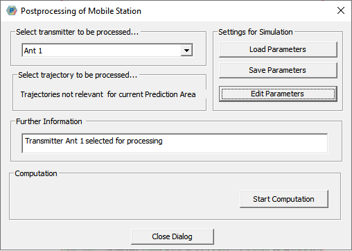
Figure 1. The Postprocessing of Mobile Station dialog.
After selecting which of the available transmitters is to be used and which of the available trajectories is to be analysed (if any), click Edit Parameters to define further options. This bring up the Settings of the Mobile Station dialog.
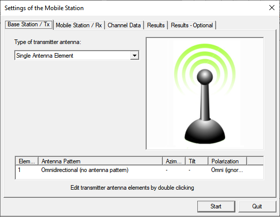
Figure 2. The Settings of the Mobile Station dialog, Mobile Station / Tx tab.
Here, the Base Station / Tx tab and the Mobile Station / Rx tab are where the MIMO antenna arrays can optionally be defined:
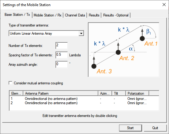
Figure 3. The Settings of the Mobile Station dialog, Mobile Station / Tx tab.
MIMO is optional, since the same dialog can be used for SISO (single input, single output).
In the lower section of the dialog, the single antenna elements within an array can be specified with an antenna pattern, azimuth and tilt adjustments. By default, all antenna elements are considered to be omnidirectional isotropic radiators. By double clicking on an antenna element, the antenna adjustment dialog opens. You can import an antenna pattern (.ffe, .apa or .apb format) and specify the location and orientation.
On the Channel Data tab, you specify how ray information is to be combined. Coherent superposition includes detailed multipath, but the visualization of small-scale fading is not always desired.
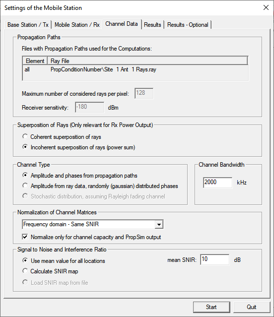
Figure 4. The Specification of the Mobile Station, Channel Data tab.
The normalization mode for the MIMO channel capacity has to be chosen, depending on the way you intend to compare the calculated capacities. For a comparison based on the same SNIR, you have to choose Same SNIR. Other options in the drop-down list include Path Loss. The mean SNIR to be considered during the channel capacity calculations has to be specified, too.
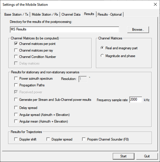
Figure 5. The Specification of the Mobile Station, Results tab.
- Results for Trajectories
-
- Doppler shift
- The Doppler shift for trajectories is written to a .txt file (for example: Site 1 Ant 1 DopplerShift_Trajectory_0_Route 0.txt).
- Doppler spread
- The Doppler spread for trajectories is written to a .txt file (for example: Site 1 Ant 1 DopplerSpread.txt).
- PROPSIM Channel Sounder (F8)
- WinProp radio channel data is exported to Keysight PROPSIM .asc file and a .shd file.
On the Results – Optional tab, you specify the optional output, see Figure 6.
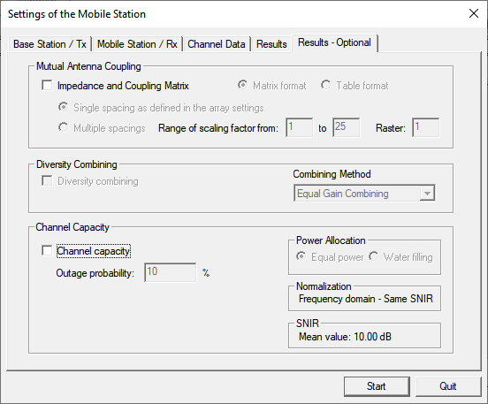
Figure 6. The Settings of the Mobile Station dialog, Results - Optional tab.
Once everything has been specified, click Start Computation to return to the Post Processing of Mobile Station dialog, see Figure 1.