Example 1: Analysis of a Rectangular Reflectarray
This case explains how to analyze a reflectarray layout. The database used on step 4 to create the reflectarray layout is the database for 37 steps and 20 divisions per wavelength (see Annex 2: Analysis of a Reflectarray Database Creation).
Step 1: Create a new MOM Project.
Open newFASANT and select 'File --> New' option.
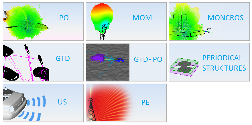
Figure 1. New Project panel
Select 'MOM' option on the previous figure and start to configure the project.
Step 2: Create the geometry model.
First, select 'millimeters' on units list on the bar at the bottom of the main window.
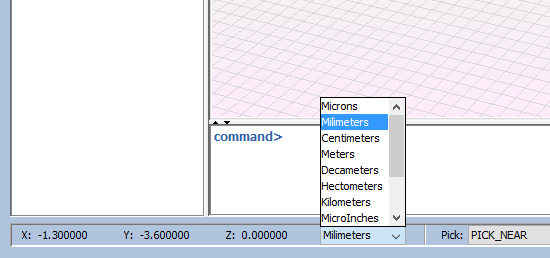
Figure 2. Units Selection
Add these parameters to have the reference for the reflectarray layout generation. On this tab, all the parameters to be used in the construction of geometry will be set (see Define Parameters). - ‘length’ contains the length value for the plane of the reflectarray layout. In order to follow the reference article, this parameter must be the length of the unitary cell of the database (x = 11.43mm) multiplied by 37 unitary cells that the reflectarray contains in ‘X’ axis. - ‘width’ contains the width value for the plane of the reflectarray layout. In order to follow the reference article, this parameter must be the width of the unitary cell of the database (y = 10.16mm) multiplied by 29 unitary cells that the reflectarray contains in ‘Y’ axis. - ‘focus’ contains the value for the position of the focus on the ‘Z’ axis. This value will be used for positioning a relative plane to locate the radiation pattern and its value is 340mm.
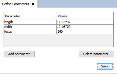
Figure 3. Define Parameters panel
Generate a plane with a width of ‘length’ and a depth of ‘width’, with the first corner on -‘length’/2, -‘width’/2, 0; executing the 'plane' command writing it on the command line and sets the parameters when command line asks for it.
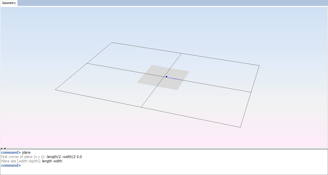
Figure 4. Plane parameters
Step 3: Set Simulation Parameters
Select 'Simulation --> Parameters' option on the menu bar and the following panel appears. Set the parameters as the next figure shows and save it.
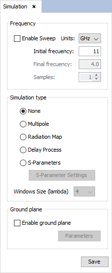
Figure 5. Simulation Parameters panel
Step 4: Create a reflectarray layout.
Select 'Source --> Reflectarray --> New Layout' option. The following panel will appear. First load de database previously created with Periodical Structures module. Then select the parameters as the next figure shows
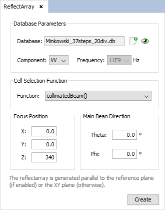
Figure 6. Reflectarray New Layout panel
Clicking on the 'eye' icon, the parameters of the database will be shown on a new tab.
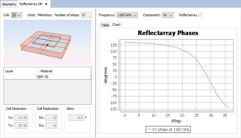
Figure 7. Reflectarray Database Information panel
Select the plane previously created to generate the reflectarray on it. Then, click on 'Create' button and wait until the reflectarray layout is created.
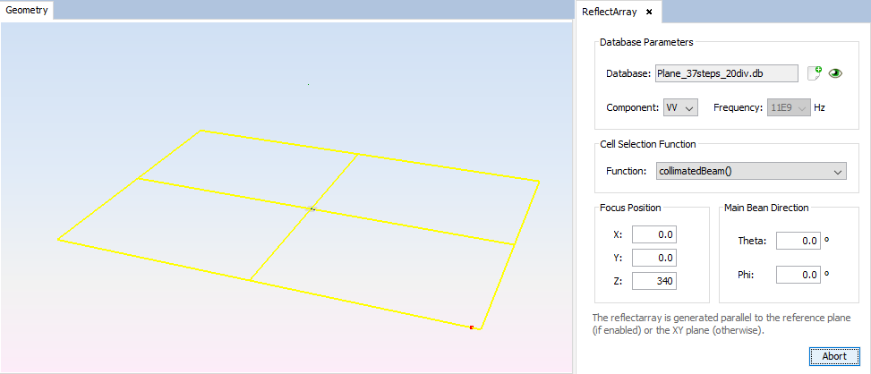
Figure 8. Reflectarray creation process
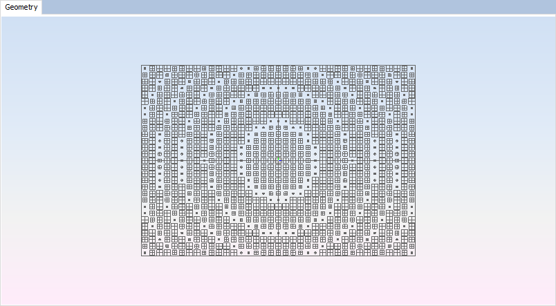
Figure 9. Reflectarray Layout
Step 5: Set the antenna parameters.
First, select 'View--> Reference Plane' and set the parameters as the next figure shows, then click on 'Update' button to put the reference plane as the figure:
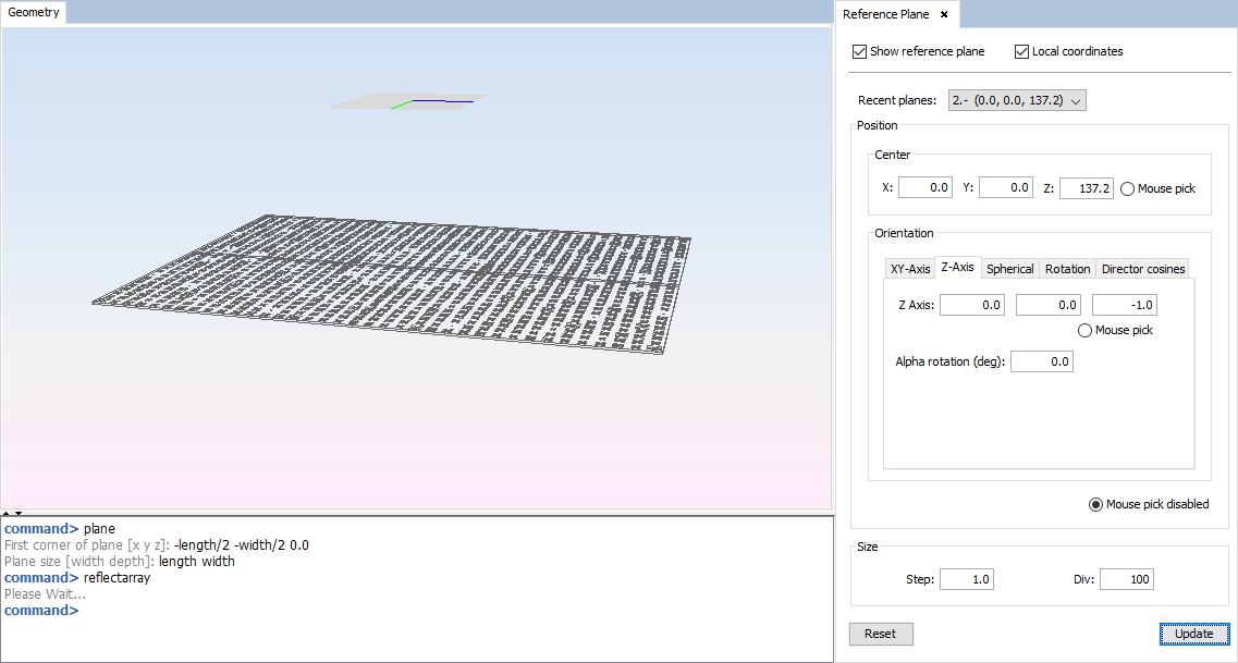
Figure 10. Reference Plane panel
Select 'Source --> Import Pattern File' option and select 'BOC0677.dia' file from 'myDataFiles' folder on the installation path of newFASANT software.
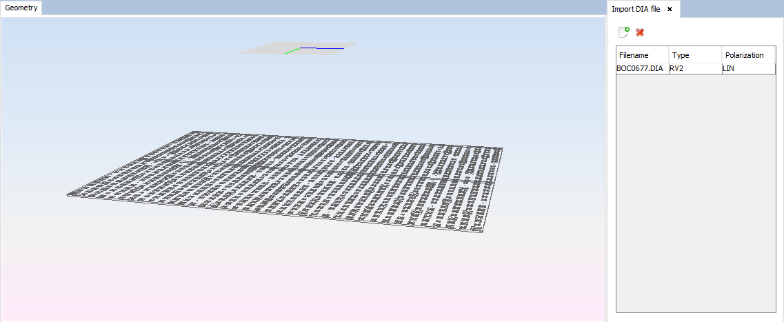
Figure 11. Pattern File Import panel
Select 'Source --> Pattern File --> Pattern File Antenna' option and set the parameters as show the next figure. Then save the parameters and the antenna appears.
Important select the check box "Relative to reference plane" to set the position and orientation relative to the local reference plane.
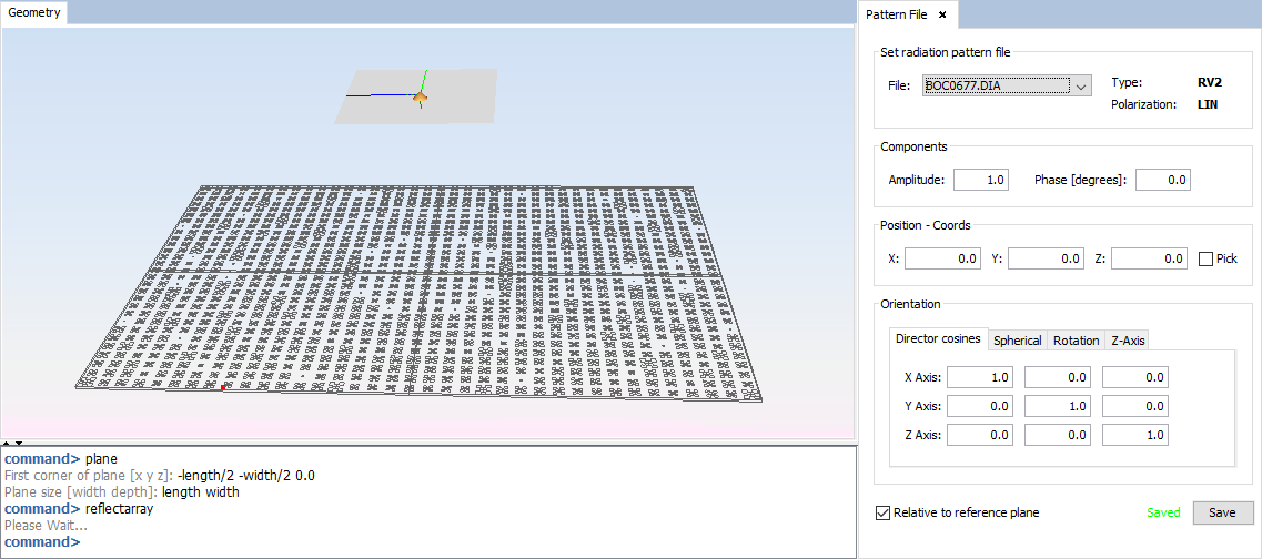
Figure 12. Pattern File Antenna panel
Step 6: Set solver parameters.
Select Solver --> Parameters' to open the solver configuration panel and then set the following parameters in order to obtain the most possible efficiency and the 3D results: - OpenMP option for the Architecture Strategy, on Solver parameters panel.
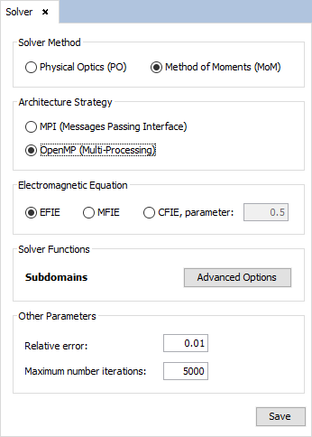
- Check the “Compute 3D Pattern” box and set the angle step to 0.5, on ‘Main Properties’ tab.
- Check the “Enable Preconditioner” box and select Diagonal Preconditioner option on ‘Preconditioner’ tab.
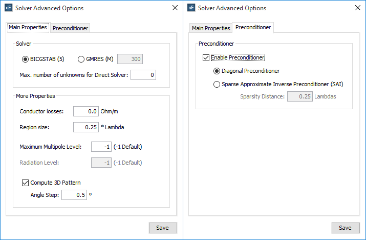
Figure 13. Solver Advanced Options panel
Step 7: Meshing the geometry model.
Select 'Meshing --> Parameters' to open the meshing configuration panel and then set the parameters as show the next figure.In this case, the number of division is selected by the case with the most accuracy of the databases compared to section Periodical Structures. The number of processors to be selected, to improve the efficiency on time, will be the number of the processors of the machine where the example will be executed.
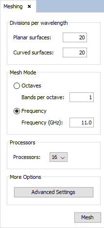
Figure 14. Meshing Parameters panel
Step 8: Execute the simulation.
Select 'Calculate --> Execute' option to open simulation parameters. Then select the number of processors as the next figure show. The number of processors to be selected, to improve the efficiency on time, will be the number of the processors of the machine where the example will be executed.
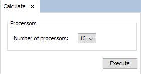
Figure 15. Execute Parameters panel
Step 9: Show Results. To get more information about the graphics panel advanced options (clicking on right button of the mouse over the panel) see Annex 1: Graphics Advanced Options.
Select 'Show Results --> Far Field --> View Cuts' option to show the cuts of the observation directions options. Delete all series with the red cross button and select 'Gain Lineal' and 'ETotal Gain (dBi)' on 'Component' panel, then click on 'Add Series' button.
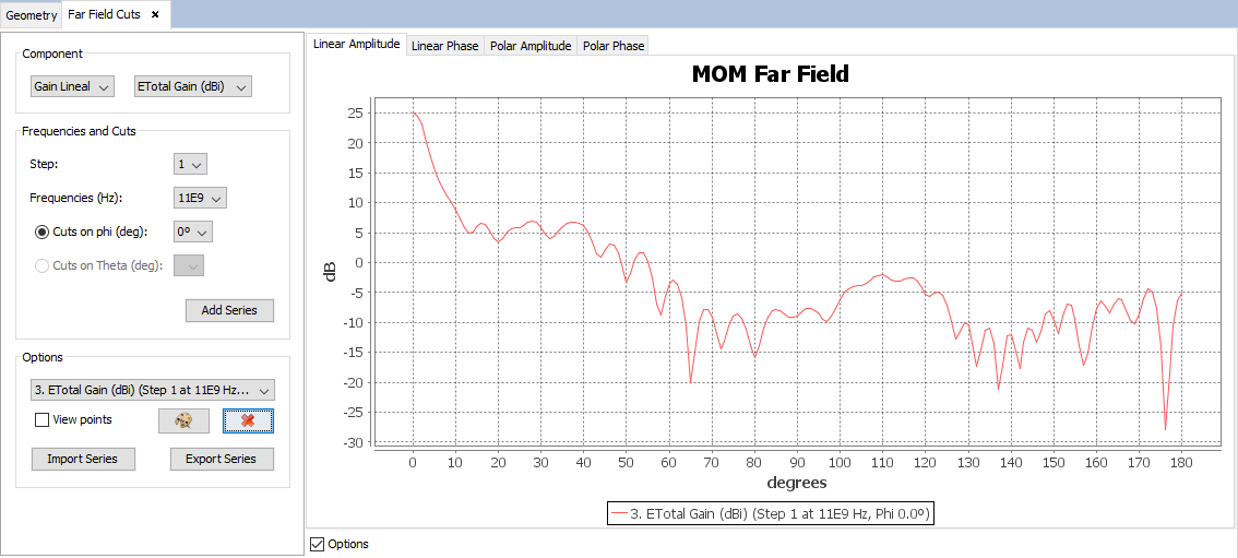
Figure 16. Far Field cuts
Selecting other values for the component, step, frequency or cut parameters and clicking on 'Add Series' button a new cut will be added to the selected parameters. On 'Show Results --> Far Field' menu, other results are present such as 'View Cuts by Step' and 'View Cuts by Frequency' and this option display the values for one selected point for each step or frequency.
Select 'Show Results --> Radiation Pattern --> View 3D Pattern' option to show the cuts of the radiation pattern options.
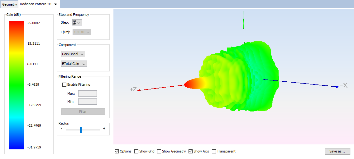
Figure 17. Radiation Pattern 3D
Changing values for step, frequency, component or filtering parameters the visualization for the new parameters will be shown.