Example 8: S-Parameters
This case explains how to calculate the S-parameters of an bifilar helix antenna placed on a plane.
Step 1 Create a new MOM Project
Open newFASANT and select File - New option. Select MOM on the module selection.
Figure 1. New Project panel
Step 2 Create the bifilar antenna with its ground plane
Open the Source menu and navigate to click on Primitive Antenna - Coaxial Feed - Helix - Multi-filar Helix option to select an antenna from the primitives.
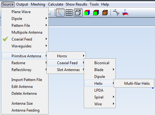
Figure 2. Primitive Antenna menu
The Multi-filar Helix panel is open on right side. Set all parameters by default except the number of Helixes, which is set to 2. Then, this primitive provide two ports defined one in each Helix. Confirm the antenna definition by clicking on Add button. After that, close the Multi-filar Helix panel.
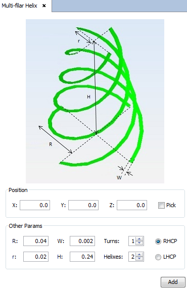
Figure 3. Bi-filar helix definition
This antenna must be placed on a planar structure which acts as reference plane. Use the plane command to insert a plane under the helix antenna with the following parameters.
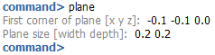
Figure 4. Plane parameters
The resulting geometry is represented in next figure.
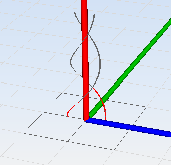
Figure 5. Final geometric design
Step 3 Set Simulation Parameters
Click on Simulation - Parameters option on the menu bar. Set a Frequency Sweep and the S-Parameters as shown in the figure below. Remember clicking on Save button to confirm the changes.
Note that a large number of frequencies has been set in this example, so the simulation time may requires several minutes. You may reduce the number of Samples to speed-up the simulation time and generate the example with less resolution.
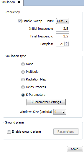
Figure 6. Simulation Parameters panel
Step 4 Set Solver Parameters
Click on Solver - Parameters option on the menu bar. Verify that all the parameters are defined by default, as shown in next figure. Click on Save button before going to next step.
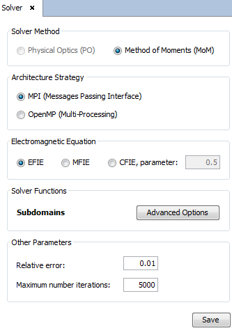
Figure 7. Solver Parameters panel
Step 5 Meshing
Click on Meshing - Create Mesh option on the menu bar. To use the same mesh for all the frequency sweep, select the Frequencyand specify the upper frequency of the range, 3.5 GHz. Select the available number of Processors, and then launch the meshing process by clicking on Mesh button.
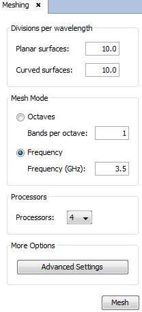
Figure 8. Meshing parameters
After the end of the meshing process, the meshes may be visualized by clicking on Meshing - Visualize Existing Mesh and select the mesh within any frequency folder. Then, you can verify that the mesh show the electrical continuity between the helix filaments and the ground plane, as shown in next figure.
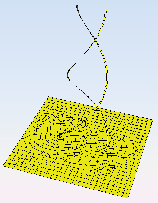
Figure 9. Generated mesh
Step 6 Execute
Click on Calculate - Execute menu and launch the simulation with the available processors. Launch the simulation by clicking on Calculate button.
Step 7 Results
When the simulation process has finished, the S-Parameters are enabled within the results menu. Click on Show Results menu and S-Parameters option to visualize this parameters. The panel with the available options to visualize the S-Parameters is open on right side.
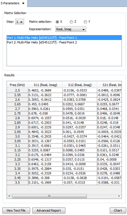
Figure 10. S-Parameters parameters
Select the S Matrix Representation and the option db, Phase in Representation section. Then, select the column to represent in the Results table and then click on Chart button to add them to plot them.
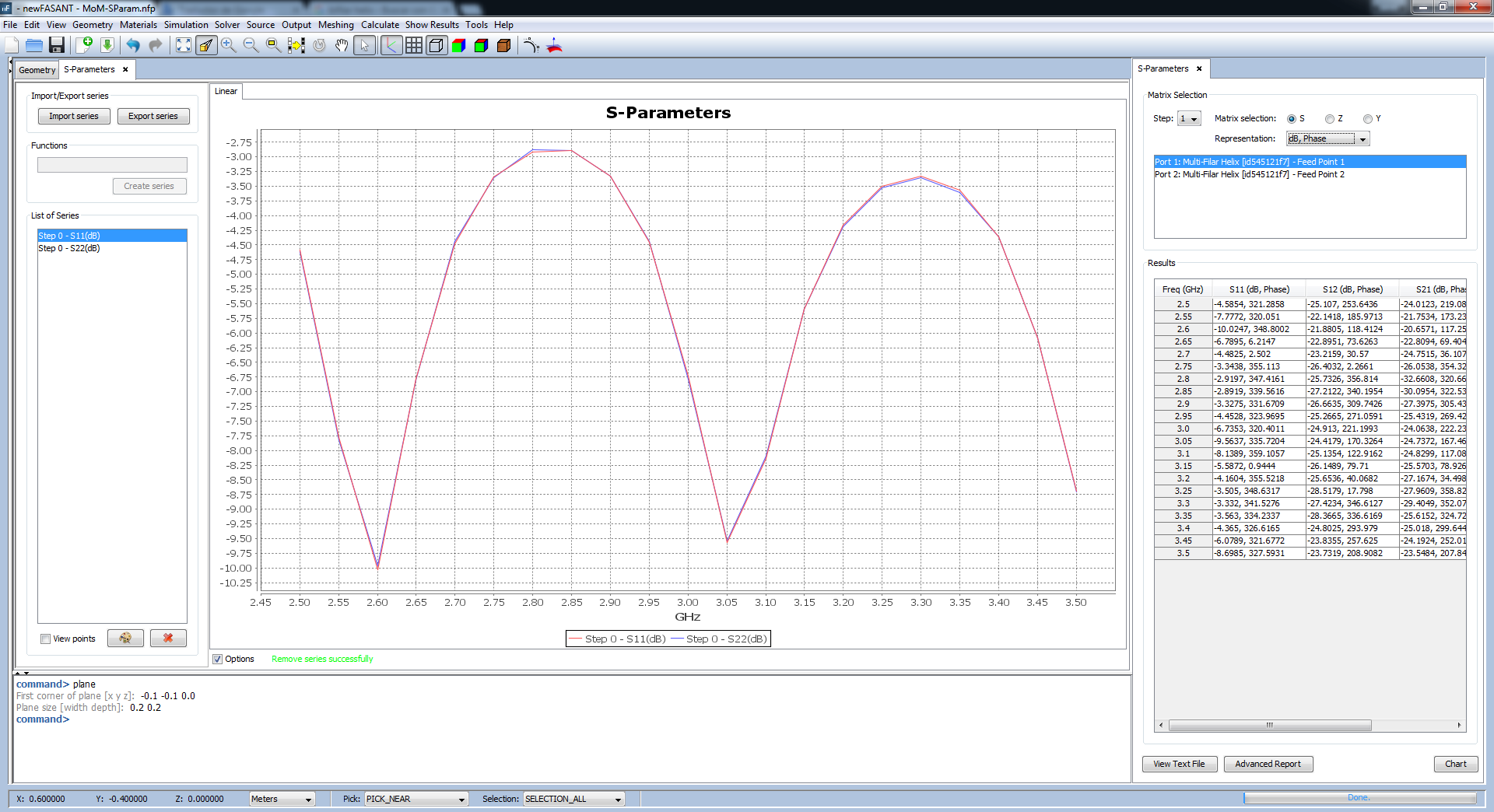
Figure 11. S11 and S22 parameters plot
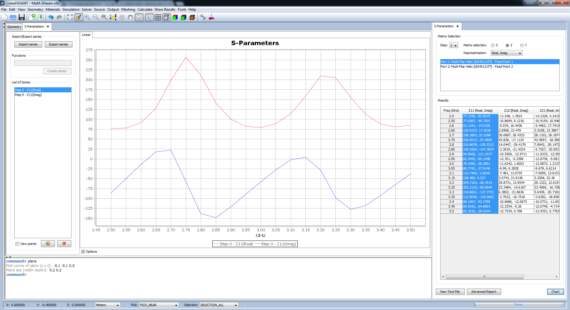
Figure 12. Z11 parameters plot
Click on Advanced Report button, and select all the fields to be exported into a html file, which may be selected in the new Advanced Report window shown in next figure.
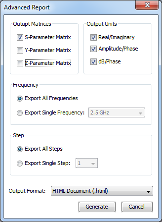
Figure 13. Advanced Report window
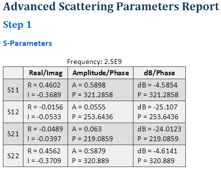
Figure 14. Advanced Report results for the first frequency